Advanced Search Algorithms for Constraint Satisfaction Problems (CSPs)

1. Constraint Satisfaction Problems Basic Algorithms My Thanks to Roman Bartak (for “stealing” some of his slides) ΑΝΑΠΑΡΑΣΤΑΣΗ ΓΝΩΣΗΣ - Lecture 1

2. Search Algorithms forCSPs • We will study variations of DFS especially forCSPs. • These algorithms are based on backtracking search Simple or Chronological Backtracking (BT) Backjumping (BJ) and Conflict-Based Backjumping Forward Checking (FC) Maintaining Arc Consistency (MAC) Also two variations of hill climbing • Min-conflicts • Min-conflicts with Random Walk ΑΝΑΠΑΡΑΣΤΑΣΗ ΓΝΩΣΗΣ - Lecture 1

3. Intelligent Backtracking • ΒΤ suffers fromthrashing • it visits again and again the same regions of the search tree becauseit has a very local view of the problem • One way to get rid of the problem is using intelligent backtracking algorithms • BJ, CBJ, DB, Graph-based BJ, Learning • Backjumping (BJ) is different from ΒΤ in the following: • When BJ reaches a dead-end it does not backtrack to the immediately preceding variables. It backtracks to the deepest variable in the search tree which is in conflict with the current variable ΑΝΑΠΑΡΑΣΤΑΣΗ ΓΝΩΣΗΣ - Lecture 1

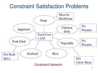
4. BJ vs. BT We want to color each area in the map with a different color We have three colors red, green, blue ΑΝΑΠΑΡΑΣΤΑΣΗ ΓΝΩΣΗΣ - Lecture 1

5. BJ vs. BT • Let’s consider what ΒΤ does in the map coloring problem • Assume that variables are assigned in the orderQ, NSW, V, T, SA, WA, NT • Assume that we have reached the partial assignment Q = red, NSW = green, V = blue, T = red • When we try to give a value to the next variableSA, we find out that all possible values violate constraints • Dead end! • BT will backtrack to try a new value for variableΤ! • Not a good idea! ΑΝΑΠΑΡΑΣΤΑΣΗ ΓΝΩΣΗΣ - Lecture 1

6. BJ vs. BT • BJ has a smarter approach to backtracking • It tells us to go back to one of the variables which are responsible for the dead-end • The set of these variables is called a conflict set • The conflict set forSA is {Q, NSW, V} • BJ backjumps to the deepest variable in theconflict set of the variable where the dead-end occurred • deepest = the one we visited most recently • CBJ, DB, Graph-based BJ, Learning, Backmarking ΑΝΑΠΑΡΑΣΤΑΣΗ ΓΝΩΣΗΣ - Lecture 1

7. Conflict-based Backjumping (CBJ) • Conflict-based Backjumping is alook-back algorithm that performs intelligent backtracking at dead-ends • In contrast toBJ whichbackjumps only from leaf dead-ends, CBJ can also backjump from dead-ends at inner nodes • for each variablex we have a conflict set • when an assignment(x,a) fails because of a constraint violation with a previous variabley, y is added to the conflict set of x • if there are no values left in the domain of the current variable x,CBJ backjumps to the deepest variable w in the conflict set of x (as BJ) • and the conflict set of x is added to the conflict set of w • then a furtherbackjump can occur fromw ΑΝΑΠΑΡΑΣΤΑΣΗ ΓΝΩΣΗΣ - Lecture 1

8. Forward Checking • Forward Checking (FC) belongs to the family of backtracking algorithms calledlookahead algorithms • The basic idea oflookahead is that when you assign a value to a variablethe problem is reduced throughconstraint propagation • constraint propagation is defined in a different way for each look-ahead algorithm • FC does the following: • When a variablex takes a valuev, for each future variabey which appears in a constraint withx we remove fromDx all the values that are not consistent withv ΑΝΑΠΑΡΑΣΤΑΣΗ ΓΝΩΣΗΣ - Lecture 1

9. Forward Checking • If the domain of some variable becomes empty thenvaluev is rejected and we try the next value ofx • The operation ofFC means that the following holds for each step of the search: • All values of eachfuture variableare compatible with all the values that have been assigned to past variables • FC maintains a restricted form ofarc consistency ΑΝΑΠΑΡΑΣΤΑΣΗ ΓΝΩΣΗΣ - Lecture 1

10. Forward Checking procedure FORWARD_CHECKING (vars,doms,cons) solution FC (vars,Ø,doms,cons) function FC (unlabelled,compound_label,doms,cons) returns a solution or NIL ifunlabelled= Øthen return compound_label else pick a variable x from unlabelled repeat pick a value v from Dx; delete v from Dx doms’ UPDATE(unlabelled-{x},doms,cons,compound_label + {(x,v)}) if no domain in doms’ is empty then result  FC(unlabelled - {x}, compound_label + {(x,v)}, doms’,cons) if result  NIL then return result end until Dx = Ø return NIL end ΑΝΑΠΑΡΑΣΤΑΣΗ ΓΝΩΣΗΣ - Lecture 1

11. Forward Checking function UPDATE (unlab_vars,doms,cons,compound_label) returns an updated set of domains for each variable y in unlab_varsdo for each value v in Dy’ do if (y,v) is incompatible with compound_label with respect to the constraints between y and the variables of compound_label then Dy’  Dy’ – {v} end end returndoms’ ΑΝΑΠΑΡΑΣΤΑΣΗ ΓΝΩΣΗΣ - Lecture 1

12. FC in operation V NSW T Q SA WA NT initial domains after WA=R after Q=G after V=B ΑΝΑΠΑΡΑΣΤΑΣΗ ΓΝΩΣΗΣ - Lecture 1

13. Consistency Techniques • removing inconsistent values from variables’ domains • graph representation of the CSP • binary and unary constraints only (relatively easy) • nodes = variables • edges = constraints • node consistency (NC) • arc consistency (AC) • path consistency (PC) • (strong) k-consistency A>5 A A<C AB C B B=C ΑΝΑΠΑΡΑΣΤΑΣΗ ΓΝΩΣΗΣ - Lecture 1

14. Node Consistency • A variableX isnode consistent iff each value a of X satisfies all the unary constraints on X • Node consistency can be applied as a preprocessing step before starting search to remove all the node inconsistent values A>5 If D(A)={0,…,9} node consistency will remove values 0,…,5 A A<C AB C B B=C ΑΝΑΠΑΡΑΣΤΑΣΗ ΓΝΩΣΗΣ - Lecture 1

15. Arc Consistency • Definition: • A variableX isarc consistent iff for each other variableYthe following holds: For each valuea ofΧthere is at least one valueb ofΥsuch thata andb are compatible • Then we say thata supportsb • An algorithm that appliesarc consistency deletes values from the domainof a variable when they are not supported by any value in the domain of another variable ΑΝΑΠΑΡΑΣΤΑΣΗ ΓΝΩΣΗΣ - Lecture 1

16. Arc Consistency (AC) • the most widely used consistency technique (good simplification/performance ratio) • deals with individual binary constraints • repeated revisions of arcs • Directional (one pass) AC a b c a b c a b c Y X Z ΑΝΑΠΑΡΑΣΤΑΣΗ ΓΝΩΣΗΣ - Lecture 1

17. AC - Example • Problem:X::{1,2}, Y::{1,2}, Z::{1,2}X = Y, X  Z, Y > Z X X 1 2 1 2 1 2 1 2 Y Y 1 2 1 2 Z Z ΑΝΑΠΑΡΑΣΤΑΣΗ ΓΝΩΣΗΣ - Lecture 1

18. 1 2 3 4 5 Arc Consistency propagation: Crossword Puzzle example ….No more changes! X1 X2 X4 astar live live load happy load peal peal hello peel peel hoses save save talk talk ΑΝΑΠΑΡΑΣΤΑΣΗ ΓΝΩΣΗΣ - Lecture 1

19. Arc Consistency • We apply arc consistency: • As a (preprocessing) step before we start search • in that way we can reduce the size of the search tree • and in some cases discover inconsistent problems • While searching after an assignment of a value to a variable • constraint propagation  fast discovery of dead ends • The search algorithm which appliesarc consistency is calledMAC (maintaining arc consistency) ΑΝΑΠΑΡΑΣΤΑΣΗ ΓΝΩΣΗΣ - Lecture 1

20. MAC procedure Maintaining Arc Consistency (vars,doms,cons) solution MAC (vars,Ø,doms,cons) function MAC (unlabelled,compound_label,doms,cons) returns a solution or NIL ifunlabelled= Øthen return compound_label else pick a variable x from unlabelled repeat pick a value v from Dx; delete v from Dx doms’ AC(unlabelled-{x},doms,cons,compound_label + {(x,v)}) if no domain in doms’ is empty then result  MAC(unlabelled - {x}, compound_label + {(x,v)}, doms’,cons) if result  NIL then return result end until Dx = Ø return NIL end ΑΝΑΠΑΡΑΣΤΑΣΗ ΓΝΩΣΗΣ - Lecture 1

21. Algorithms forArc Consistency • Arc consistency can be enforced with Ο(ed2) optimal worst case time complexity • AC-4, AC-6, AC-7, AC-2001 • AC-3: non-optimal,but simpleAC algorithm • AC-3 andAC-2001 use: • a queue (or stack) where the variables that are checked for arc consistency are inserted • a routineRevise which deletes values that are not supported • AC-4, AC-6, AC-7 use more complex data structures • support lists ΑΝΑΠΑΡΑΣΤΑΣΗ ΓΝΩΣΗΣ - Lecture 1

22. Achieving Arc Consistency • From Mackworth (1977a): procedureAC-3(G) Let Q be the set of (directed) arcs of G (not self-cyclic) while Q not empty do select and remove any arc (x,y) from Q; REVISE(x,y) if REVISE(x,y) changed the domain of x then add to Q the set of all arcs of G (z,x) that go into x; procedureREVISE(x,y) for each value a in domain of x do if there is no value b in the domain of y such that (a,b) is consistent then delete a from the domain of x ΑΝΑΠΑΡΑΣΤΑΣΗ ΓΝΩΣΗΣ - Lecture 1

23. Achieving Arc Consistency • Runtime of AC-3: O(ed3) for graph e binary constraints, and maximum domain size ofd • For one constraint, function Revise costs O(d2) and it can be called d times • there are e constraints, so the complexity is O(ed3) • AC-2001/3.1 achievesthe optimal Ο(ed2) complexity by using a set of pointers Lastx,a,y • For each value a of a variable, Lastx,a,y points to the most recently discovered value in the domain of y that supports a procedureREVISE-2001/3.1(x,y) for each value a in domain of x do if there is no value b in the domain of y such that b> Lastx,a,y and (a,b) is consistent then delete a from the domain of x else Lastx,a,y = first such value ΑΝΑΠΑΡΑΣΤΑΣΗ ΓΝΩΣΗΣ - Lecture 1

24. Algorithms for Arc Consistency • In some cases we can exploit the semantics of certain binary constraints to achieve an even better complexity • functional, anti-functional, monotonic, piecewise functional, etc. • algorithm AC-5 • What the complexity of AC processing for a constraint of the following types? • x = y • x ≠ y • x < y • x > y ΑΝΑΠΑΡΑΣΤΑΣΗ ΓΝΩΣΗΣ - Lecture 1

25. Directional Arc Consistency (DAC) • Observation:AC has to repeat arc revisions; the totalnumber of revisions depends on the number of arcs butalso on the size of domains (while cycle) • Is it possible to weaken AC in such a way that every arc isrevised just once? • Definition: A CSP is directional arc consistentusing a givenorder of variables iff every arc (i,j) such that i<j is arcconsistent • Again, every arc has to be revised, but revision in onedirection is enough now ΑΝΑΠΑΡΑΣΤΑΣΗ ΓΝΩΣΗΣ - Lecture 1

26. Arc Consistency as a Solution Method • Question: • Are there cases where we can guarantee that solubility (or insolubility) will be determined by applying arc consistency? • Answer (Freuder 1982): • When the constraint graph of the problem is a tree • In this case, a solution can be found (if one exists) in a backtrack-free manner by first applying directional arc consistency • A case of polynomially solvable CSPs • Many other such cases exist depending on the structure of the constraint graph and the nature of the constraints ΑΝΑΠΑΡΑΣΤΑΣΗ ΓΝΩΣΗΣ - Lecture 1

27. Is AC enough? • empty domain => no solution • cardinality of all domains is 1 => solution • Problem:X::{1,2}, Y::{1,2}, Z::{1,2}X  Y, X  Z, Y  Z X 1 2 1 2 Y Z 1 2 ΑΝΑΠΑΡΑΣΤΑΣΗ ΓΝΩΣΗΣ - Lecture 1

28. Stronger Levels ofConsistency • Beyondarc consistency there are numerous other levels ofconsistency • path consistency • singleton arc consistency • neighborhood inverse consistency • … • These are stronger thanarc consistency (i.e. they delete more inconsistent values when they are applied) • But they are more expensive (higher time complexity) • We will review some of them in the next lecture ΑΝΑΠΑΡΑΣΤΑΣΗ ΓΝΩΣΗΣ - Lecture 1

29. Constraint Propagation • systematic search only => no efficient • consistency only => no complete • combination of search (backtracking) with consistency techniques • methods: • look back (restoring from conflicts) • look ahead (preventing conflicts) look back look ahead Labelling order ΑΝΑΠΑΡΑΣΤΑΣΗ ΓΝΩΣΗΣ - Lecture 1

30. Look Back Methods • intelligent backtracking • consistency checks among instantiated variables • backjumping • backtracks to the conflicting variable • backchecking and backmarking • avoids redundant constraint checkingby remembering conflicting levelfor each value jump here a conflict b b b still conflict ΑΝΑΠΑΡΑΣΤΑΣΗ ΓΝΩΣΗΣ - Lecture 1

31. Look Ahead Methods • preventing future conflicts via consistency checks among not yet instantiated variables • forward checking (FC) • AC to direct neighbourhood • partial look ahead (PLA) • DAC • (full) look ahead (LA) • Arc Consistency • Path Consistency instantiated variable labelling order ΑΝΑΠΑΡΑΣΤΑΣΗ ΓΝΩΣΗΣ - Lecture 1

32. Look Ahead - Example • Problem:X::{1,2}, Y::{1,2}, Z::{1,2}X = Y, X  Z, Y > Z generate & test - 7 stepsbacktracking - 5 stepspropagation - 2 steps ΑΝΑΠΑΡΑΣΤΑΣΗ ΓΝΩΣΗΣ - Lecture 1

33. Q1 Q2 Q3 Q4 1 2 3 4 Qi: line number of queen in column i, for 1i4 Q1, Q2, Q3, Q4 Q1Q2, Q1Q3, Q1Q4, Q2Q3, Q2Q4, Q3Q4, Q1Q2-1, Q1Q2+1, Q1Q3-2, Q1Q3+2, Q1Q4-3, Q1Q4+3, Q2Q3-1, Q2Q3+1, Q2Q4-2, Q2Q4+2, Q3Q4-1, Q3Q4+1 4-queen problem Place 4 queens so that no two queens are in attack. ΑΝΑΠΑΡΑΣΤΑΣΗ ΓΝΩΣΗΣ - Lecture 1

34. Q1 Q2 Q3 Q4 1 2 3 4 There is a total of 256 valuations GT algorithm will generate 64 valuations with Q1=1; + 48 valuations with Q1=2, 1Q23; + 3 valuations with Q1=2, Q2=4, Q3=1; = 115 valuations to find first solution 4-queen problem first solution ΑΝΑΠΑΡΑΣΤΑΣΗ ΓΝΩΣΗΣ - Lecture 1

35. Q1 Q2 Q3 Q4 Q1 Q2 Q3 Q4 1 1 2 2 3 3 4 4 Q1 Q2 Q3 Q4 1 2 3 4 Q1 Q2 Q3 Q4 Q1 Q2 Q3 Q4 1 1 2 2 3 3 4 4 4-queen problem, BT algorithm ΑΝΑΠΑΡΑΣΤΑΣΗ ΓΝΩΣΗΣ - Lecture 1

36. Q1 Q2 Q3 Q4 Q1 Q2 Q3 Q4 1 1 2 2 3 3 4 4 Q1 Q2 Q3 Q4 Q1 Q2 Q3 Q4 1 1 2 2 3 3 4 4 Q1 Q2 Q3 Q4 Q1 Q2 Q3 Q4 Q1 Q2 Q3 Q4 1 1 1 2 2 2 3 3 3 4 4 4 4-queen problem, FC algorithm ΑΝΑΠΑΡΑΣΤΑΣΗ ΓΝΩΣΗΣ - Lecture 1

37. Q1 Q2 Q3 Q4 1 2 x 3 x 4 x Q1 Q2 Q3 Q4 Q1 Q2 Q3 Q4 Q1 Q2 Q3 Q4 1 1 1 2 2 2 3 3 3 4 4 4 4-queen problem, MAC algorithm Value 3 of Q2 is unsupported in Q3, Value 4 of Q3 is unsupported in Q2, Value 2 of Q3 is unsupported in Q4, ΑΝΑΠΑΡΑΣΤΑΣΗ ΓΝΩΣΗΣ - Lecture 1

38. Hybrid Algorithms • We can combine the operations of various backtracking algorithms to designhybrid algorithms • For examplewe can combine thelookahead function offorward checking and thelookback function ofBJ • FC-BJ • FC-CBJ • MAC-BJ • MAC-CBJ • … ΑΝΑΠΑΡΑΣΤΑΣΗ ΓΝΩΣΗΣ - Lecture 1

39. FC-CBJ • Forward Checking with Conflict-based Backjumping • FC-CBJ combines the look-ahead of FC and the intelligent backjumping of CBJ • each variable is associated with a conflict set • when the forward checking of an assignment (x,a) results in a value deletion from the domain of a variable y, x is added to the conflict set of y • if after the forward checking of an assignment (x,a) the domain of a variable y is wiped out, the variables in the conflict set of y are added to the conflict set of x • why is this done? • if there are no more values left in the domain of the current variable x, FC-CBJ backjumps to the deepest variable w in the conflict set of x • the conflict set of x is added to the conflict set of w ΑΝΑΠΑΡΑΣΤΑΣΗ ΓΝΩΣΗΣ - Lecture 1

40. Evaluation of Backtracking Algorithms • How can we compare backtracking algorithms forCSPs ? • Time / Space Complexity • not very useful. They all have exponential time complexity! • cpu times • number of nodes they visit in the search tree • amount ofconsistency checks they perform • amount of backtracks they perform ΑΝΑΠΑΡΑΣΤΑΣΗ ΓΝΩΣΗΣ - Lecture 1

41. Evaluation of Backtracking Algorithms • Some theoretical results: • Search tree nodes visited FC-CBJ  FC-BJ  FC  BJ  BT CBJ  BJ • Number of consistency checks CBJ  BJ ΒΤ FC-CBJ  FC-BJ  FC • CPU times ? We always need experiments!!! ΑΝΑΠΑΡΑΣΤΑΣΗ ΓΝΩΣΗΣ - Lecture 1

42. Heuristic Methods forCSPs • Search algorithms must take decisions: • Which will be the next variable to assign ? • Which value should I give it ? • Which constraint should I check ? • The decisions that the algorithm takes at each step have a drastic effect on the search space (and the efficiency of the algorithm) • Especially decision (1) • Heuristics help the algorithms take correct decisions • fail first principle ΑΝΑΠΑΡΑΣΤΑΣΗ ΓΝΩΣΗΣ - Lecture 1

43. Heuristic Methods forCSPs • Variable ordering heuristics • static heuristics • MaxDegree, Bandwidth, … • dynamic heuristics • MRV, Brelaz, dom/deg, dom/wdeg… • Value ordering heuristics • Geelen’s promise, least-constraining… • Heuristics for constraint ordering • based on the cost of propagation ΑΝΑΠΑΡΑΣΤΑΣΗ ΓΝΩΣΗΣ - Lecture 1

44. Variable Ordering Heuristics • Minimum Width • The width of a variable x is the number of variables that are before x, according to a given ordering, and are constrained with x • The width of an ordering is the maximum width of all the variables under that ordering • The width of a constraint graph is the minimum width of all possible orderings • Variables are ordered in descending width • useful when the degree of the nodes varies significantly • Problem: How many are the possible orderings? ΑΝΑΠΑΡΑΣΤΑΣΗ ΓΝΩΣΗΣ - Lecture 1

45. Variable Ordering Heuristics • Maximum Degree • Variables are ordered in decreasing order of their degree in the constraint graph • degree is the number of adjacent variables in the graph • Heuristic to find a minimum width ordering • Maximum Cardinality • Selects the first variable arbitrarily • Then, at each stage, selects the variable that is adjacent to the largest set of already selected variables. ΑΝΑΠΑΡΑΣΤΑΣΗ ΓΝΩΣΗΣ - Lecture 1

46. Variable Ordering Heuristics • Minimum Bandwidth • The bandwidth of a variable x, according to a given ordering, is the maximum distance between x and any other variable which is adjacent to x • The bandwidth of an ordering is the maximum bandwidth of all the variables under that ordering • The bandwidth of a constraint graph is the minimum bandwidth of all possible orderings • Idea: The closer the variables involved in a constraint are placed to each other the less backtracking will be required • Problem: Computing the minimum bandwidth is NP-complete ΑΝΑΠΑΡΑΣΤΑΣΗ ΓΝΩΣΗΣ - Lecture 1

47. Dynamic Variable Ordering Heuristics • Minimum Remaining Values (MRV) or Smallest Domain (SD) • At each stage of search select the variable with the smallest domain size • How do we break ties? • Select a variable randomly • Select the variable with the highest degree in the original graph • Select the variable with the highest future degree (i.e. the one involved in the maximum number of constraints with future variables). This is called the Brelaz heuristic • Many variations have been proposed • dom/deg, dom/fdeg ΑΝΑΠΑΡΑΣΤΑΣΗ ΓΝΩΣΗΣ - Lecture 1

48. State-of-the-art Dynamic Variable Ordering Heuristics • Weighted degree heuristics • each constraint is associated with a weight initially set to 1 • each time a constraint c removes the last value from a domain (i.e. causes a domain wipeout - DWO) its weight is incremented by 1 • the weighted degree of a variable x is the sum of the weights of the constraints that include x • wdeg heuristic • selects the variable with maximum weighted degree • dom/wdeg heuristic • selects the variable with minimum ration of domain size to weighted degree • What is the rationale behind these heuristics? • they use information gathered throughout search – not just from the current search state like dom/fdeg ΑΝΑΠΑΡΑΣΤΑΣΗ ΓΝΩΣΗΣ - Lecture 1

49. Value Ordering Heuristics • Min-Conflicts • Associate with each value a the total number of values in future variables that are incompatible with a • Select the value with lowest sum • Alternative: Divide the number of incompatible values of future variable x with the domain size of x • Geelen’s Promise • For each value a count the total number of values in each future variable that are compatible with a • Take the product of the counts. This is called the promise of value a • Select the value with the maximum promise ΑΝΑΠΑΡΑΣΤΑΣΗ ΓΝΩΣΗΣ - Lecture 1

50. Constraint Ordering Heuristics • Is this issue important? • not very much when maintaining arc consistency • but there exist heuristics for ordering the constraints in the propagation queue. Can you think of such a heuristic? • but very important in modern advanced solvers that use propagators for the various (global) constraints • the idea here is to propagate the less expensive constraints first ΑΝΑΠΑΡΑΣΤΑΣΗ ΓΝΩΣΗΣ - Lecture 1