Understanding OLS: Theoretical Foundations, Assumptions, and Applications in Econometrics
This comprehensive review delves into Ordinary Least Squares (OLS) by exploring its theoretical underpinnings, key assumptions, and practical applications in econometrics. Key assumptions such as linearity, exogeneity, no multicollinearity, homoscedasticity, and the implications of non-spherical disturbances are discussed. The review further elaborates on the least squares estimator, variance-covariance matrices, and asymptotic normality, providing a clear framework for understanding OLS. Practical examples, including an exploration of the U.S. gasoline market, illustrate real-world applications of these concepts.

Understanding OLS: Theoretical Foundations, Assumptions, and Applications in Econometrics
E N D
Presentation Transcript
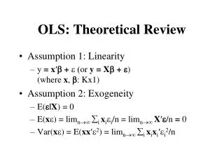
OLS: Theoretical Review • Assumption 1: Linearity • y = x′b + e(or y = Xb + e) (where x, b: Kx1) • Assumption 2: Exogeneity • E(|X) = 0 • E(x) = limn i xiei/n = limn X′/n = 0 • Var(x) = E(xx′2) = limn i xixi′ei2/n
OLS: Theoretical Review • Assumption 3: No Multicolinearity • rank(X) = K • E(xx') = limnixixi′/n = limnX′X/n • plim X’X/n exists and nonsingular
OLS: Theoretical Review • Non-Spherical Disturbances: General Heteroschedasticity • Var(e) = • Var(xe) = E(xx′e2) = limnX′X/n • X′e/n dN(0,X′X/n)
OLS: Theoretical Review • Assumption 4: Homoschedasticity andNo Autocorrelation • Var(e) = s2I • Var(xe) = E(xx′e2) = limns2X′X/n • X′e/n dN(0, s2X′X/n)
OLS: Theoretical Review • Least Squares Estimator • b = (X'X)-1X'y • Variance-Covariance Matrix of b • General Heteroscedasticity:Var(b) = (X'X)-1X′X(X'X)-1 • Homoschedasticity: Var(b) = 2(X'X)-1
OLS: Theoretical Review • Least Squares Estimator • b = (X'X/n)-1(X'y/n) • b = + (X'X/n)-1(X'/n), bp • n(b - ) = (X'X/n)-1(X'/n) • n(b - ) dN(0,A-1BA-1)A = E(xx′) = limnX'X/nB = E(xx′e2) = limnX'X/n • n(b - ) dN(0, s2A-1) under homoschedasticity
OLS: Theoretical Review • Asymptotic Normality • b ~aN(, (X'X)-1X′X(X'X)-1) • b ~aN(, s2(X'X)-1) under homoschedasticity • The unknown or s2 needs to be consistently estimated.
OLS: Theoretical Review • Estimate of Asymptotic Var(b) • Under Homoschedasticity
OLS: Theoretical Review • Estimate of Asymptotic Var(b) • White Estimator (Heteroschedasticity-Consistent Estmate of Asymptotic Covariance Matrix)
OLS: Theoretical Review • GLS (Generalized Least Squares) • If is known and nonsingular, then -1/2 y = -1/2 X + -1/2 or y* = X* + * • E(*|X*) = 0, E(**'|X*) = I • bGLS = (X'-1X)-1X'-1y • Var(bGLS) = (X'-1X)-1 • bGLS ~aN(, (X'-1X)-1)
Example • U. S. Gasoline Market, 1953-2004 • EXPG = Total U.S. gasoline expenditure • PG = Price index for gasoline • Y = Per capita disposable income • Pnc = Price index for new cars • Puc = Price index for used cars • Ppt = Price index for public transportation • Pd = Aggregate price index for consumer durables • Pn = Aggregate price index for consumer nondurables • Ps = Aggregate price index for consumer services • Pop = U.S. total population in thousands
Example • y = Xb + e • y = G; X = [1 PG Y]where G = (EXPG/PG)/POP • y = ln(G); X = [1 ln(PG) ln(Y)] • Elasticity Interpretation