
Constraint satisfaction problems
E N D
Presentation Transcript
Constraint satisfaction problems CS171, Fall 2016 Introduction to Artificial Intelligence Prof. Alexander Ihler
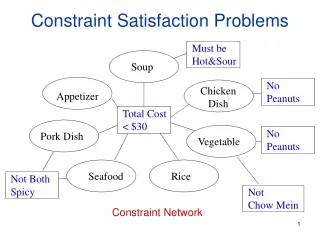
Constraint Satisfaction Problems • What is a CSP? • Finite set of variables, X1, X2, …, Xn • Nonempty domain of possible values for each: D1, ..., Dn • Finite set of constraints, C1...Cm • Each constraint Ci limits the values that variables can take, e.g., X1 X2 • Each constraint Ci is a pair: Ci = (scope, relation) • Scope = tuple of variables that participate in the constraint • Relation = list of allowed combinations of variables May be an explicit list of allowed combinations May be an abstract relation allowing membership testig & listing • CSP benefits • Standard representation pattern • Generic goal and successor functions • Generic heuristics (no domain-specific expertise required)
Example: Sudoku • Problem specification 1 2 3 4 5 6 7 8 9 A B C D E F G H I Variables: {A1, A2, A3, … I7, I8, I9} Domains: { 1, 2, 3, … , 9 } Constraints: each row, column “all different” alldiff(A1,A2,A3…,A9), ... each 3x3 block “all different” alldiff(G7,G8,G9,H7,…I9), ... Task: solve (complete a partial solution) check “well-posed”: exactly one solution?
CSPs: What is a Solution? • State: assignment of values to some or all variables • Assignment is complete when every variable has an assigned value • Assignment is partial when one or more variables have no assigned value • Consistent assignment • An assignment that does not violate any constraint • A solution to a CSP is a complete and consistent assignment • All variables are assigned, and no constraints are violated • CSPs may require a solution that maximizes an objective • Linear objective ) linear programming or integer linear programming • Ex: “Weighted” CSPs • Examples of applications • Scheduling the time of observations on the Hubble Space Telescope • Airline schedules • Cryptography • Computer vision, image interpretation
Example: Map Coloring Variables: Domains: { red, green, blue } Constraints: bordering regions must have different colors: A solution is any setting of the variables that satisfies all the constraints, e.g.,
Example: Map Coloring • Constraint graph • Vertices: variables • Edges: constraints (connect involved variables) • Graphical model • Abstracts the problem to a canonical form • Can reason about problem through graph connectivity • Ex: Tasmania can be solved independently (more later) • Binary CSP • Constraints involve at most two variables • Sometimes called “pairwise”
Aside: Graph coloring • More general problem than map coloring • Planar graph: graph in 2D plane with no edge crossings • Guthrie’s conjecture (1852) Every planar graph can be colored · 4 colors • Proved (using a computer) in 1977 (Appel & Haken 1977)
Varieties of CSPs • Discrete variables • Finite domains, size d ) O(dn) complete assignments • Ex: Boolean CSPs: Boolean satisfiability (NP-complete) • Inifinite domains (integers, strings, etc.) • Ex: Job scheduling, variables are start/end days for each job • Need a constraint language, e.g., StartJob_1 + 5 · StartJob_3 • Infinitely many solutions • Linear constraints: solvable • Nonlinear: no general algorithm • Continuous variables • Ex: Building an airline schedule or class schedule • Linear constraints: solvable in polynomial time by LP methods
Varieties of constraints • Unary constraints involve a single variable, • e.g., SA ≠ green • Binary constraints involve pairs of variables, • e.g., SA ≠ WA • Higher-order constraints involve 3 or more variables, • Ex: jobs A,B,C cannot all be run at the same time • Can always be expressed using multiple binary constraints • Preference (soft constraints) • Ex: “red is better than green” can often be represented by a cost for each variable assignment • Combines optimization with CSPs
Simplify… • We restrict attention to: • Discrete & finite domains • Variables have a discrete, finite set of values • No objective function • Any complete & consistent solution is OK • Solution • Find a complete & consistent assignment • Example: Sudoku puzzles
Binary CSPs CSPs only need binary constraints! • Unary constraints • Just delete values from the variable’s domain • Higher order (3 or more variables): reduce to binary • Simple example: 3 variables X,Y,Z • Domains Dx={1,2,3}, Dy={1,2,3}, Dz={1,2,3} • Constraint C[X,Y,Z] = {X+Y=Z} = {(1,1,2),(1,2,3),(2,1,3)} (Plus other variables & constraints elsewhere in the CSP) • Create a new variable W, taking values as triples (3-tuples) • Domain of W is Dw={(1,1,2),(1,2,3),(2,1,3)} • Dw is exactly the tuples that satisfy the higher-order constraint • Create three new constraints: • C[X,W] = { [1,(1,1,2)], [1,(1,2,3)], [2,(2,1,3) } • C[Y,W] = { [1,(1,1,2)], [2,(1,2,3)], [1,(2,1,3) } • C[Z,W] = { [2,(1,1,2)], [3,(1,2,3)], [3,(2,1,3) } Other constraints elsewhere involving X,Y,Z are unaffected
Example: Cryptarithmetic problems • Find numeric substitutions that make an equation hold: T W O + T W O = F O U R Non-pairwise CSP: O+O = R + 10*C1 C1 = {0,1} For example: O = 4 R = 8 W = 3 U = 6 T = 7 F = 1 all-different W+W+C1 = U + 10*C2 7 3 4 + 7 3 4 = 1 4 6 8 C2 = {0,1} F T U O W R T+T+C2 = O + 10*C3 C3 = {0,1} C1 C3 C2 C3 = F Note: not unique – how many solutions?
Example: Cryptarithmetic problems • Try it yourself at home: (a frequent request from college students to parents) S E N D + M O R E = M O N E Y
(adapted from http://www.unitime.org/csp.php) Random binary CSPs • A random binary CSP is defined by a four-tuple (n, d, p1, p2) • n = the number of variables. • d = the domain size of each variable. • p1 = probability a constraint exists between two variables. • p2 = probability a pair of values in the domains of two variables connected by a constraint is incompatible. • Note that R&N lists compatible pairs of values instead. • Equivalent formulations; just take the set complement. • (n, d, p1, p2) generate random binary constraints • The so-called “model B” of Random CSP (n, d, n1, n2) • n1 = p1 n(n-1)/2 pairs of variables are randomly and uniformly selected and binary constraints are posted between them. • For each constraint, n2 = p2 d^2 randomly and uniformly selected pairs of values are picked as incompatible. • The random CSP as an optimization problem (minCSP). • Goal is to minimize the total sum of values for all variables.
CSP as a standard search problem • A CSP can easily be expressed as a standard search problem. • Incremental formulation • Initial State: the empty assignment {} • Actions: Assign a value to an unassigned variable provided that it does not violate a constraint • Goal test: the current assignment is complete (by construction it is consistent) • Path cost: constant cost for every step (not really relevant) • Aside: can also use complete-state formulation • Local search techniques (Chapter 4) tend to work well BUT: solution is at depth n (# of variables) For BFS: branching factor at top level is nd next level: (n-1)d … Total: n! dnleaves! But there are only dncomplete assignments!
Commutativity • CSPs are commutative. • Order of any given set of actions has no effect on the outcome. • Example: choose colors for Australian territories, one at a time. • [WA=red then NT=green] same as [NT=green then WA=red] • All CSP search algorithms can generate successors by considering assignments for only a single variable at each node in the search tree there are dn irredundant leaves • (Figure out later to which variable to assign which value.)
Backtracking search • Similar to depth-first search • At each level, pick a single variable to expand • Iterate over the domain values of that variable • Generate children one at a time, one per value • Backtrack when a variable has no legal values left • Uninformed algorithm • Poor general performance
Backtracking search (R&N Fig. 6.5) function BACKTRACKING-SEARCH(csp) return a solution or failure return RECURSIVE-BACKTRACKING({} , csp) function RECURSIVE-BACKTRACKING(assignment, csp) return a solution or failure ifassignment is complete then return assignment var SELECT-UNASSIGNED-VARIABLE(VARIABLES[csp],assignment,csp) for each value in ORDER-DOMAIN-VALUES(var, assignment, csp)do ifvalue is consistent with assignment according to CONSTRAINTS[csp] then add {var=value} to assignment result RECURSIVE-BACTRACKING(assignment, csp) if result failure then return result remove {var=value} from assignment return failure
Backtracking search • Expand deepest unexpanded node • Generate only onechild at a time. • Goal-Test when inserted. • For CSP, Goal-test at bottom Future= green dotted circles Frontier=white nodes Expanded/active=gray nodes Forgotten/reclaimed= black nodes
Backtracking search • Expand deepest unexpanded node • Generate only onechild at a time. • Goal-Test when inserted. • For CSP, Goal-test at bottom Future= green dotted circles Frontier=white nodes Expanded/active=gray nodes Forgotten/reclaimed= black nodes
Backtracking search • Expand deepest unexpanded node • Generate only onechild at a time. • Goal-Test when inserted. • For CSP, Goal-test at bottom Future= green dotted circles Frontier=white nodes Expanded/active=gray nodes Forgotten/reclaimed= black nodes
Backtracking search • Expand deepest unexpanded node • Generate only onechild at a time. • Goal-Test when inserted. • For CSP, Goal-test at bottom Future= green dotted circles Frontier=white nodes Expanded/active=gray nodes Forgotten/reclaimed= black nodes
Backtracking search • Expand deepest unexpanded node • Generate only onechild at a time. • Goal-Test when inserted. • For CSP, Goal-test at bottom Future= green dotted circles Frontier=white nodes Expanded/active=gray nodes Forgotten/reclaimed= black nodes
Backtracking search • Expand deepest unexpanded node • Generate only onechild at a time. • Goal-Test when inserted. • For CSP, Goal-test at bottom Future= green dotted circles Frontier=white nodes Expanded/active=gray nodes Forgotten/reclaimed= black nodes
Backtracking search • Expand deepest unexpanded node • Generate only onechild at a time. • Goal-Test when inserted. • For CSP, Goal-test at bottom Future= green dotted circles Frontier=white nodes Expanded/active=gray nodes Forgotten/reclaimed= black nodes
Backtracking search • Expand deepest unexpanded node • Generate only onechild at a time. • Goal-Test when inserted. • For CSP, Goal-test at bottom Future= green dotted circles Frontier=white nodes Expanded/active=gray nodes Forgotten/reclaimed= black nodes
Backtracking search • Expand deepest unexpanded node • Generate only onechild at a time. • Goal-Test when inserted. • For CSP, Goal-test at bottom Future= green dotted circles Frontier=white nodes Expanded/active=gray nodes Forgotten/reclaimed= black nodes
Backtracking search • Expand deepest unexpanded node • Generate only onechild at a time. • Goal-Test when inserted. • For CSP, Goal-test at bottom Future= green dotted circles Frontier=white nodes Expanded/active=gray nodes Forgotten/reclaimed= black nodes
Backtracking search • Expand deepest unexpanded node • Generate only onechild at a time. • Goal-Test when inserted. • For CSP, Goal-test at bottom Future= green dotted circles Frontier=white nodes Expanded/active=gray nodes Forgotten/reclaimed= black nodes
Backtracking search • Expand deepest unexpanded node • Generate only onechild at a time. • Goal-Test when inserted. • For CSP, Goal-test at bottom Future= green dotted circles Frontier=white nodes Expanded/active=gray nodes Forgotten/reclaimed= black nodes
Backtracking search (R&N Fig. 6.5) function BACKTRACKING-SEARCH(csp) return a solution or failure return RECURSIVE-BACKTRACKING({} , csp) function RECURSIVE-BACKTRACKING(assignment, csp) return a solution or failure ifassignment is complete then return assignment var SELECT-UNASSIGNED-VARIABLE(VARIABLES[csp],assignment,csp) for each value in ORDER-DOMAIN-VALUES(var, assignment, csp)do ifvalue is consistent with assignment according to CONSTRAINTS[csp] then add {var=value} to assignment result RECURSIVE-BACTRACKING(assignment, csp) if result failure then return result remove {var=value} from assignment return failure
Improving Backtracking O(exp(n)) • Make our search more “informed” (e.g. heuristics) • General purpose methods can give large speed gains • CSPs are a generic formulation; hence heuristics are more “generic” as well • Before search: • Reduce the search space • Arc-consistency, path-consistency, i-consistency • Variable ordering (fixed) • During search: • Look-ahead schemes: • Detecting failure early; reduce the search space if possible • Which variable should be assigned next? • Which value should we explore first? • Look-back schemes: • Backjumping • Constraint recording • Dependency-directed backtracking
Look-ahead: Variable and value orderings • Intuition: • Apply propagation at each node in the search tree (reduce future branching) • Choose a variable that will detect failures early (low branching factor) • Choose value least likely to yield a dead-end (find solution early if possible) • Forward-checking • (check each unassigned variable separately) • Maintaining arc-consistency (MAC) • (apply full arc-consistency)
Dependence on variable ordering • Example: coloring Color WA, Q, V first: 9 ways to color none inconsistent (yet) only 3 lead to solutions… Color WA, SA, NT first: 6 ways to color all lead to solutions no backtracking
Dependence on variable ordering • Another graph coloring example:
Minimum remaining values (MRV) • A heuristic for selecting the next variable • a.k.a. most constrained variable (MCV) heuristic • choose the variable with the fewest legal values • will immediately detect failure if X has no legal values • (Related to forward checking, later)
Degree heuristic • Another heuristic for selecting the next variable • a.k.a. most constraining variable heuristic • Select variable involved in the most constraints on other unassigned variables • Useful as a tie-breaker among most constrained variables What about the order to try values?
Least Constraining Value • Heuristic for selecting what value to try next • Given a variable, choose the least constraining value: • the one that rules out the fewest values in the remaining variables • Makes it more likely to find a solution early
Variable and value orderings • Minimum remaining values for variable ordering • Least constraining value for value ordering • Why do we want these? Is there a contradiction? • Intuition: • Choose a variable that will detect failures early (low branching factor) • Choose value least likely to yield a dead-end (find solution early if possible) • MRV for variable selection reduces current branching factor • Low branching factor throughout tree = fast search • Hopefully, when we get to variables with currently many values, forward checking or arc consistency will have reduced their domains & they’ll have low branching too • LCV for value selection increases the chance of success • If we’re going to fail at this node, we’ll have to examine every value anyway • If we’re going to succeed, the earlier we do, the sooner we can stop searching
Summary • CSPs • special kind of problem: states defined by values of a fixed set of variables, goal test defined by constraints on variable values • Backtracking = depth-first search with one variable assigned per node • Heuristics • Variable ordering and value selection heuristics help significantly • Variable ordering (selection) heuristics • Choose variable with Minimum Remaining Values (MRV) • Degree Heuristic – break ties after applying MRV • Value ordering (selection) heuristic • Choose Least Constraining Value
Constraint satisfaction problems(continued) CS171, Fall 2016 Introduction to Artificial Intelligence Prof. Alexander Ihler
You Should Know • Node consistency, arc consistency, path consistency, K-consistency (6.2) • Forward checking (6.3.2) • Local search for CSPs • Min-Conflict Heuristic (6.4) • The structure of problems (6.5)
Minimum remaining values (MRV) • A heuristic for selecting the next variable • a.k.a. most constrained variable (MCV) heuristic • choose the variable with the fewest legal values • will immediately detect failure if X has no legal values • (Related to forward checking, later) Idea: reduce the branching factor now Smallest domain size = fewest # of children = least branching
Detailed MRV example WA=red Initially, all regions have |Di|=3 Choose one randomly, e.g. WA & pick value, e.g., red (Better: tie-break with degree…) Do forward checking (next topic) NT & SA cannot be red Now NT & SA have 2 possible values – pick one randomly
Detailed MRV example NT=green NT & SA have two possible values Choose one randomly, e.g. NT & pick value, e.g., green (Better: tie-break with degree; select value by least constraining) Do forward checking (next topic) SA & Q cannot be green Now SA has only 1 possible value; Q has 2 values.
Detailed MRV example SA=blue SA has only one possible value Assign it Do forward checking (next topic) Now Q, NSW, V cannot be blue Now Q has only 1 possible value; NSW, V have 2 values.
Degree heuristic • Another heuristic for selecting the next variable • a.k.a. most constraining variable heuristic • Select variable involved in the most constraints on other unassigned variables • Useful as a tie-breaker among most constrained variables Note: usually (& in picture above) we use the degree heuristic as a tie-breaker for MRV; however, in homeworks & exams we may use it without MRV to show how it works. Let’s see an example.
Ex: Degree heuristic (only) • Select variable involved in largest # of constraints with other un-assigned vars • Initially: degree(SA) = 5; assign (e.g., red) • No neighbor can be red; we remove the edges to assist in counting degree • Now, degree(NT) = degree(Q) = degree(NSW) = 2 • Select one at random, e.g. NT; assign to a value, e.g., blue • Now, degree(NSW)=2 • Idea: reduce branching in the future • The variable with the largest # of constraints will likely knock out the most values from other variables, reducing the branching factor in the future SA=red NT=blue NSW=blue
Ex: MRV + degree • Initially, all variables have 3 values; tie-breaker degree => SA • No neighbor can be red; we remove the edges to assist in counting degree • Now, WA, NT, Q, NSW, V have 2 values each • WA,V have degree 1; NT,Q,NSW all have degree 2 • Select one at random, e.g. NT; assign to a value, e.g., blue • Now, WA and Q have only one possible value; degree(Q)=1 > degree(WA)=0 • Idea: reduce branching in the future • The variable with the largest # of constraints will likely knock out the most values from other variables, reducing the branching factor in the future SA=red NT=blue NSW=blue
Least Constraining Value • Heuristic for selecting what value to try next • Given a variable, choose the least constraining value: • the one that rules out the fewest values in the remaining variables • Makes it more likely to find a solution early