Download
1 / 50
520 likes | 814 Vues
Novel Designs in Phase I Trials: A guide to scientifically acceptable and simple designs. Rick Chappell, Ph.D. Professor, Department of Biostatistics and Medical Informatics and Department of Statistics University of Wisconsin School of Medicine and Public Health Stat 641, Fall 2010.

E N D
Novel Designs in Phase I Trials:A guide to scientifically acceptable and simple designs. Rick Chappell, Ph.D. Professor, Department of Biostatistics and Medical Informatics and Department of Statistics University of Wisconsin School of Medicine and Public Health Stat 641, Fall 2010
Outline • Existing Phase I Designs • Introduction • “Traditional” Design • Storer’s “Up-and-Down” Designs • Two-Stage Designs • Accelerated Titration • Combined Outcomes (Phase I/II Designs) • Continual Reassessment Method • General Design Considerations • (Designs for Long-Term Toxicities) • (Linked Phase I Trials) • Conclusion
Outline • Existing Phase I Designs • Introduction • “Traditional” Design • Storer’s “Up-and-Down” Designs • Two-Stage Designs • Accelerated Titration • Combined Outcomes (Phase I/II Designs) • Continual Reassessment Method • General Design Considerations • (Designs for Long-Term Toxicities) • (Linked Phase I Trials) • Conclusion } “Novel Designs”
1. Introduction • Goal first delineated by Schneiderman (1967) as estimation of dose yielding a fixed percent (often 33%) of dose-limiting toxicities (DLTs) but not lower. This is called the Maximum Tolerable Dose (MTD).
Phases of a Clinical Trial • Biochemical and pharmacological research. • Animal Studies (Gart, 1986 & Schneiderman, 1967). • Phase I, Cancer (Storer, 1989) - estimate toxicity rates using few (~ 10 - 40) typically very sick subjects. • Phase II (Thall & Simon, 1995) - determines a therapy’s potential efficacy using a few very sick patients.
Phases of a Clinical Trial (cont.) • Phase III – a large randomized controlled, possibly blinded, possibly multicenter, experiment • Phase IV - a controlled trial of an approved treatment with long-term followup of safety and efficacy.
Schematic of Phase I Trial 100 % Toxicity 33 . . . mtd 0 d1 d2 Dose
Allowable DLT rate can be lower than 33% but rarely higher 100 % Toxicity 20 .. mtd 0 d1 d2 Dose
2. “Traditional” Designs • Groups of three; dose increased (only) until some stopping criterion is achieved. • “Designed” to estimate the MTD as 33%-ile or the next-largest dose. • Underestimates the MTD. • Not flexible (can spend a lot of patients at low-toxicity doses).
3. “Up-and-Down” Designs • Groups of three or less. • Dose levels increased and/or decreased until a predetermined sample size is reached. • Designed to estimate the MTD as 33%-ile, as before. • Not flexible (can also spend a lot of patients at low-toxicity doses), but can easily be modified to speed up.
Storer’s (1989) simple phase I up-and-down classification Design A (“Traditional”): Groups of three patients are treated. Escalation occurs if no toxicity is observed in all three: otherwise, an additional three patients are treated at the same dose level. If only one of six has toxicity, escalation again continues; otherwise, the trial stops. Design B: Single patients are treated. The next patient is treated at the next lower dose level if a toxic response is observed, otherwise at the next higher dose level until sample size is reached.
Design D: Groups of three patients are treated. Escalation if no toxicity is seen and de-escalation if more than one patient has toxicity. If one patient has toxicity, next group of three is treated at same dose level; repeat until sample size is reached. Similar to traditional except can go down. ( Design C: Similar to design D, except that the rule applies to the preceding three patients at any point, instead of using discrete batches of three. ) Note these designs center around the dose with 1/3 = 33% toxicity rate. Larger cohorts can be used to estimate the MTD as the dose with a 1/4 = 25%, 1/5 = 20% or 1/6 = 17% rates.
Problems with the “Traditional Design”: Storer and DeMets (1987) gave a clear illustration of bias potential in a phase I trial using the traditional stopping rule (“Design A”). Due to the multiple opportunities for stopping, it stops too early and does not re-escalate. The stopping dose is not the 33rd %-ile - it is lower. But we don’t know how much lower:
Dose Actual (Unknown) Pr (Stopping) Level Percentile at D.L. 1 .15 19% 2 .20 24% 3 .25 23% 4 .30 18% 5 .33 10% “Even if dose level 5 corresponds exactly to the 33rd percentile, the probability (computed from the third column) that this particular trial will ever reach it is only 17%.”
Problems with the “Traditional Design” - Cohorts of size 3 or 6 may tell you less than you think: What can you learn from 3 patients at a single dose? What is the 95% exact c.i. for the probability of toxicity at a given dose if you observe • 0/3 toxicities at that dose? • 1/3 toxicities at that dose? • 2/3 toxicities at that dose? • 3/3 toxicities at that dose?
Problems with the “Traditional Design” - Cohorts of size 3 or 6 may tell you less than you think: What can you learn from 3 patients at a single dose? What is the 95% exact c.i. for the probability of toxicity at a given dose if you observe • 0/3 toxicities at that dose? ( 0, .63) • 1/3 toxicities at that dose? (.01, .90) • 2/3 toxicities at that dose? (.10, .99) • 3/3 toxicities at that dose? (.37, 1) See “confint.R” file for code to calculate these.
Problems with the “Traditional Design” - Cohorts of size 3 or 6 may tell you less than you think: What can you learn from 6 patients at a single dose? What is the 95% exact c.i. for the probability of toxicity at a given dose if you observe • 0/6 toxicities at that dose? • 1/6 toxicities at that dose? • 2/6 toxicities at that dose? • 3/6 toxicities at that dose?
Problems with the “Traditional Design” - Cohorts of size 3 or 6 may tell you less than you think: What can you learn from 6 patients at a single dose? What is the 95% exact c.i. for the probability of toxicity at a given dose if you observe • 0/6 toxicities at that dose? ( 0, .39) • 1/6 toxicities at that dose? (.005, .63) • 2/6 toxicities at that dose? (.05, .77) • 3/6 toxicities at that dose? (.12, .88)
Problems with the “Traditional Design” - Conclusion • Single or double cohorts tell you little about a dose unless it is revisited. • Thus most biostatisticians prefer more flexible up-and-down designs (e.g., Storer’s “D”).
4. Two Stage Designs(Storer, 1989): • A fast initial stage (one-at-a-time assignment), pursued until a toxicity is found; • Then assignment proceeds in groups of three until a predetermined sample size is reached. • Designed to estimate the MTD as 33%-ile. • Can use B followed by D (one-at-a-time escalation until DLT, or even grade 2 toxicity, followed by up-and-down with cohorts of 3).
5. Accelerated Titration(Simon, et al., 1999) • “Rapid intrapatient dose escalation … in order to reduce the number of undertreated patients [in the trials themselves] and provide a substantial increase in the information obtained.” • If a first dose does not induce toxicity, a patient may be escalated to a higher subsequent dose. • Obviously requires toxicities to be acute. • If they are, trial can be shortened.
Accelerated Titration (continued) • After MTD is determined, a final “confirmatory” cohort is treated at a fixed dose. • Jordan, et al. (2003) studied intrapatient escalation of carboplatin in ovarian cancer patients and found “The median MTD documented here using intrapatient dose escalation ... is remarkably similar to that derived from conventional phase I studies.” I.e., accelerated titration seems to work. Also, since it gives an MTD for each patient, it provides an idea about how MTDs vary between patients.
6. Combined Outcomes(Gooley, et al. [1994], Thall and Russell [1998], Huang and Chappell [2008] and Braun [2002]): • Designed to give simultaneous information on efficacy and toxicity. • Situation may be logically symmetrical (e.g., graft vs. host / rejection in bone marrow transplantation). • May have three ordered outcomes (best to worst): • Efficacy+, Toxicity- • Efficacy+, Toxicity+ or Efficacy-, Toxicity+ • Efficacy-, Toxicity+ • Sometimes called “Phase I/II”.
Gooley’s scenario for immunosuppression after bone-marrow transplant
7.Continual Reassessment Method – CRM (O’Quigley, et al.) Prior guess is made as to the dose-response (toxicity) curve; First patient is assigned to the prior MTD; After the patient is fully followed, his or her outcome is used to update the prior curve; Next patient is assigned to the new “posterior” MTD; Repeated until sample size is reached.
The dose-response curve is parameterized with slope β, so that Pr(Toxicity at level dk) = F(dk, β) . F is usually very simple with scalar β such as a power function (how can we get away with this?) The current dose dn is chosen such that F(dn , β) ≤ p and F(dk, β) > p for all k > n, where p is the toxicity level which defines the MTD.
Inference on β is based on the likelihood where yiis the indicator of toxic response for the ith patient and [i] is the dose level assigned to him. If desired, the likelihood can be combined with prior information for a Bayesian analysis.
Advantages of the CRM It is highly flexible: Can estimate any quantile, not just .33; Allows groups of any size; Can be modified to allow incomplete information (here). Can incorporate restrictions.
Disadvantages of the CRM Escalation rules are not intuitive or known in advance - “black box”; Requires prior information or initial escalation strategy; Extra rules required (limits on number of doses escalated per patient; starting dose lower than that dictated by the prior) for ethical considerations; The prior may need to be modified for appropriate operating characteristics.
8.Other Bayesian Designs • The Bayesian paradigm is a natural one for Phase I/II trials because of their exploratory nature and the limited number of patients available. • Babb, et al. (1998) proposed “Escalation with Overdose Control” (EWOC). • It also is designed to approach the MTD, but requires that the predicted number of patients who could exceed the MTD does not exceed a small proportion. Rules aimed at protecting patients from toxicity rather than estimating MTD.
B. Practical Considerations1. Choosing Doses Consider all possibilities!: a) What if you start at “dose 1” and it is toxic? • Stop, conclude agent is unsafe; or • De-escalate to prespecified “dose 0”. • If latter, what if “dose 0” is toxic? • If you want to de-escalate, all doses or the rules for determining them should be stated in the protocol.
1. Choosing Doses (continued) b) What if your highest dose appears nontoxic? • Stop, designate highest dose MTD; or • Continue escalating. • If latter, all doses or the rules for determining them should be stated in the protocol.
1. Choosing Doses (continued) c) What if one dose appears toxic and the next lower one elicits no toxicities? • Stop, designate the lower dose MTD; or • Choose an intermediate dose. • If latter, all doses or the rules for determining them should be stated in the protocol. • Choice may depend of route of administration (oral vs. IV).
2. Defining the DLT a) Specify your own definition - Grade 3 isn’t written in stone. Possible exceptions: • Grade 3 neutropenia not DLT (reversible)? • Grade 3 radiation pneumonitis requiring < 2 weeks oxygen not DLT (transitory)? • Grade 2 late post-radiation rectal bleeding is a DLT (irreversible)? b) Also, don’t forget to specify time frame of DLT.
3. Escalation rules a) If at all possible, de-escalate and re-escalate to a fixed sample size (e.g., with rules “C” or “D”). b) Consider intrapatient escalation (accelerated titration) when feasible. c) Consider rapid initial escalation (e.g., rule “B” until an initial toxicity is seen, then “D”) when ethical. d) Consider using additional information (e.g., rapid initial escalation in absence of grade 2 toxicities). e) Consider adding 6-15 patients at final dose.
C. Designs for Long-term Toxicities • When looking for long-term or chronic toxicities all of the above designs take a long time, even with rapid accrual. • Suppose investigators are interested in toxicities over a span of (say) two years. • For a study with only 15 patients, “three-at-a-time” designs require 10 years to complete, even with perfect accrual.
Since sequential (one-at-a-time or three-at-a-time, etc.) methods take so long in such cases, other designs should be considered. • The following scenario assumes that we are interested in the MTD as the 20%-ile of a toxicity which requires 2 years followup (so we now have cohorts of 5, not 3).
Prorated Designs (Cheung & Chappell, 2000) • Instead of collecting data on a group of 5 patients for 2 years each, • Collect data on more than 5 patients for a total of 10 patient-years. • One patient measured for one year counts (is “prorated” as) 1/2 of a patient. • A Bayesian version (TIme-To-Event Continual Reassment Method, TITE-CRM, is available).
Prorated Designs (continued): • Require more patients than traditional designs, provide more information at study’s conclusion; and • Are much quicker than traditional designs (commensurate with the number of extra patients).
Proration Example - Dose-per-fraction Escalation in Prostate Cancer • Trial under way with spiral tomoradiotherapy at UWCCC with M. Ritter and M. Mehta. • Uses result of Teshima (1997) that the incidence of grade 2 rectal complications is roughly constant within first 2 years. • Teshima’s results also show that 2-year rate is close to final one.
MTD is defined as dose which yields at most a 20% rate of grade 2 rectal toxicity at 2 years. • Escalation requires: • At least 10 patient-years of observation; • At most a 20% toxicity rate per two years (I.e., at most 1 toxicity per 10 patient-years); • A minimum of 5 patients followed for a full year, for safety’s sake. • Study duration is roughly halved.
Study Schema – Phase I/II,Split-level nested escalation/condensation
D. “Linked” Phase I Trials What happens if you have 2 or more “linked” phase I trials? • Suppose you run phase I trials in 5 groups at different levels of risk such that: • Pr(Toxicity | group 1, dose=d) • … • Pr(Toxicity | group 5, dose=d)?
Example: Radiotherapy in lung cancer, risk level = volume irradiated (Mehta, et al., 2001). • There are 5 “bins” with total lung volume irradiated 0-19%, 20-39%, … , 80-100%. • What happens if a high risk group escalates dose past that in a low risk group(s)? • E.g., what if MTD among high-volume patients exceeds that for patients with lower irradiation volumes? • Solution: pool adjacent violating bins.
Current MTD From: In its simplest form, the PAV algorithm just takes the average of conflicting results High Low Intermediate Risk Group (based on volume irradiated)
Current MTD To: In its simplest form, the PAV algorithm just takes the average of conflicting results High Low Intermediate Risk Group (based on volume irradiated)
E. Conclusion These are all examples of tailoring the design to the science. “One size fits all” doesn’t work for phase III trials. Why should it work for phase I? Pick your design to simply and ethically answer your unique question.
"I guess I should warn you that if I turn out to be particularly clear, you've probably misunderstood me.“ Alan Greenspan at his 1988 confirmation hearings.
0 0 1 1 2 2 3 3 4 4 LLN* ULN* 1000/mm3 Death 3 x ULN 6 x ULN 500/mm3 Death 1500/mm3 1.5 x ULN Example of Toxicity Grades • Neutrophil (white blood cell count) • Renal Toxicity (creatinine level) 5 5 L(U)LN: lower (upper) range of normal limit