Download

1 / 44
440 likes | 462 Vues
Understand the implementation and complexity of Sequential ATPG, covering time-frame expansion, 9-valued logic, and cycle-free circuits. Examples and methods explained. Lecture held in Prague on May 22, 2010.

E N D
TSS@ETS10Fault Models, Fault Simulation and Test Generation Vishwani D. Agrawal Department of ECE, Auburn University Auburn, AL 36849, USA www.ece.auburn.edu/~vagrawal vagrawal@eng.auburn.edu Prague, May 22, 2010, 2:30-6:30PM May 22, 2010, Agrawal: Lecture 5 Sequential ATPG
Sequential ATPG • Problem of sequential circuit ATPG • Time-frame expansion • Nine-valued logic • ATPG implementation and drivability • Complexity of ATPG • Cycle-free and cyclic circuits • Asynchronous circuits* • Simulation-based ATPG • Summary • Problems to solve * Not discussed; see M. L. Bushnell and V. D. Agrawal, Essentials of Electronic Testing for Digital, Memory and Mixed-Signal VLSI Circuits, Springer, 2000, Chapter 8. May 22, 2010, Agrawal: Lecture 5 Sequential ATPG
Sequential Circuits • A sequential circuit has memory in addition to combinational logic. • Test for a fault in a sequential circuit is a sequence of vectors, which • Initializes the circuit to a known state • Activates the fault, and • Propagates the fault effect to a primary output • Methods of sequential circuit ATPG • Time-frame expansion methods • Simulation-based methods May 22, 2010, Agrawal: Lecture 5 Sequential ATPG
Example: A Serial Adder Bn An 1 1 s-a-0 D 1 1 D X Cn Cn+1 X 1 Combinational logic Sn X FF May 22, 2010, Agrawal: Lecture 5 Sequential ATPG
Time-Frame Expansion Bn-1 An-1 Bn An Time-frame -1 Time-frame 0 1 1 1 1 s-a-0 s-a-0 D X D D 1 1 D 1 Cn-1 X D 1 Cn 1 Cn+1 X 1 Combinational logic Combinational logic 1 Sn-1 Sn X D FF May 22, 2010, Agrawal: Lecture 5 Sequential ATPG
Concept of Time-Frames • If the test sequence for a single stuck-at fault contains n vectors, • Replicate combinational logic block n times • Place fault in each block • Generate a test for the multiple stuck-at fault using combinational ATPG with 9-valued logic Vector -n+1 Vector -1 Vector 0 Fault Unknown or given Init. state Next state State variables Time- frame 0 Time- frame -n+1 Time- frame -1 Comb. block PO -1 PO 0 PO -n+1 May 22, 2010, Agrawal: Lecture 5 Sequential ATPG
Example for Logic Systems FF1 B A FF2 s-a-1 May 22, 2010, Agrawal: Lecture 5 Sequential ATPG
Five-Valued Logic (Roth)0,1, D, D, X A 0 A 0 s-a-1 s-a-1 D D X X X FF1 FF1 X D D FF2 FF2 B B X X Time-frame 0 Time-frame -1 May 22, 2010, Agrawal: Lecture 5 Sequential ATPG
Nine-Valued Logic (Muth)0,1, 1/0, 0/1,1/X, 0/X, X/0, X/1, X A 0 A X s-a-1 s-a-1 X/1 0/1 0/X 0/X X FF1 FF1 0/1 X X/1 FF2 FF2 B B X 0/1 Time-frame 0 Time-frame -1 May 22, 2010, Agrawal: Lecture 5 Sequential ATPG
Implementation of ATPG • Select a primary output (PO) reachable from fault site. • Place a logic value, 1/0 or 0/1, depending on fault type and number of inversions between fault site and PO. • Justify the output value from PIs, considering all necessary paths and adding backward time-frames. • If justification is impossible, then select another PO and repeat justification. • If the procedure fails for all reachable POs, then the fault is untestable. • If 1/0 or 0/1 cannot be justified at any PO, but 1/X or 0/X can be justified, the fault is potentially detectable. May 22, 2010, Agrawal: Lecture 5 Sequential ATPG
Complexity of ATPG • Synchronous circuit – All flip-flops controlled by clocks; PI and PO synchronized with clock: • Cycle-free circuit – No feedback among flip-flops: Test generation for a fault needs no more than dseq + 1 time-frames, where dseq is the sequential depth. • Cyclic circuit – Contains feedback among flip-flops: May need 9Nff time-frames, where Nff is the number of flip-flops. • Asynchronous circuit – Higher complexity! Time- Frame max-1 Time- Frame max-2 Time- Frame -2 Time- Frame -1 Time- Frame 0 Smax S2 S1 S0 S3 max = Number of distinct vectors with 9-valued elements= 9Nff May 22, 2010, Agrawal: Lecture 5 Sequential ATPG
Cycle-Free Circuits • Characterized by absence of cycles among flip-flops and a sequential depth, dseq. • dseq is the maximum number of flip-flops on any path between PI and PO. • Both good and faulty circuits are initializable. • Test sequence length for a fault is bounded by dseq + 1. May 22, 2010, Agrawal: Lecture 5 Sequential ATPG
F2 2 F3 F1 3 Level = 1 Cycle-Free Example Circuit F2 2 All faults are testable in this circuit. F3 F1 3 Level = 1 s - graph dseq = 3 May 22, 2010, Agrawal: Lecture 5 Sequential ATPG
Cyclic Circuit Example Modulo-3 counter Z CNT F2 F1 s - graph F2 F1 May 22, 2010, Agrawal: Lecture 5 Sequential ATPG
Modulo-3 Counter • Cyclic structure – Sequential depth is undefined. • Circuit is not initializable. No tests can be generated for any stuck-at fault. • After expanding the circuit to 9Nff = 81, or fewer, time-frames ATPG program calls any given target fault untestable. • Circuit can only be functionally tested by multiple observations. • Functional tests, when simulated, give no fault coverage. May 22, 2010, Agrawal: Lecture 5 Sequential ATPG
s - graph F2 F1 Adding Initializing Hardware Initializable modulo-3 counter Z CNT F2 F1 s-a-0 s-a-1 CLR s-a-1 s-a-1 Untestable fault Potentially detectable fault May 22, 2010, Agrawal: Lecture 5 Sequential ATPG
Benchmark Circuits Circuit PI PO FF Gates Structure Seq. depth Total faults Detected faults Potentially detected faults Untestable faults Abandoned faults Fault coverage (%) Fault efficiency (%) Max. sequence length Total test vectors Gentest CPU s (Sparc 2) s1494 8 19 6 647 Cyclic -- 1506 1379 2 30 97 91.6 93.4 28 559 19183 s1238 14 14 18 508 Cycle-free 4 1355 1283 0 72 0 94.7 100.0 3 308 15 s1196 14 14 18 529 Cycle-free 4 1242 1239 0 3 0 99.8 100.0 3 313 10 s1488 8 19 6 653 Cyclic -- 1486 1384 2 26 76 93.1 94.8 24 525 19941 May 22, 2010, Agrawal: Lecture 5 Sequential ATPG
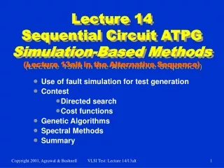
Simulation-Based ATPG • Use of fault simulation for test generation • Contest • Directed search • Cost functions • Genetic Algorithms • Spectral Methods May 22, 2010, Agrawal: Lecture 5 Sequential ATPG
Motivation • Difficulties with time-frame method: • Long initialization sequence • Impossible to guarantee initialization with three-valued logic* • Circuit modeling limitations • Timing problems – tests can cause races/hazards • High complexity • Inadequacy for asynchronous circuits • Advantages of simulation-based methods • Advanced fault simulation technology • Accurate simulation model exists for verification • Variety of tests – functional, heuristic, random • Used since early 1960s * See M. L. Bushnell and V. D. Agrawal, Essentials of Electronic Testing for Digital, Memory and Mixed-Signal VLSI Circuits, Springer, 2000, Section 5.3.4. May 22, 2010, Agrawal: Lecture 5 Sequential ATPG
A Test Causing Race X C’ A’ 1 s-a-1 A C X 1 s-a-1 B’ Z’ 1/0 0 Z B 1 Time-frame -1 Time-frame 0 Test is a two-vector sequence: X0, 11 10, 11 is a good test; no race in fault-free circuit 00, 11 causes a race condition in fault-free circuit May 22, 2010, Agrawal: Lecture 5 Sequential ATPG
Using Fault Simulator Vector source: Functional (test-bench), Heuristic (walking 1, etc.), Weighted random, random Generate new trial vectors No Trial vectors Stopping criteria (fault coverage, CPU time limit, etc.) satisfied? Fault simulator Fault list Yes Restore circuit state Update fault list New faults detected? Yes Test vectors Stop No Append vectors May 22, 2010, Agrawal: Lecture 5 Sequential ATPG
Background • Seshu and Freeman, 1962, Asynchronous circuits, parallel fault simulator, single-input changes vectors. • Breuer, 1971, Random sequences, sequential circuits • Agrawal and Agrawal, 1972, Random vectors followed by D-algorithm, combinational circuits. • Shuler, et al., 1975, Concurrent fault simulator, random vectors, sequential circuits. • Parker, 1976, Adaptive random vectors, combinational circuits. • Agrawal, Cheng and Agrawal, 1989, Directed search with cost-function, concurrent fault simulator, sequential circuits. • Srinivas and Patnaik, 1993, Genetic algorithms; Saab, et al., 1996; Corno, et al., 1996; Rudnick, et al., 1997; Hsiao, et al., 1997. May 22, 2010, Agrawal: Lecture 5 Sequential ATPG
Contest • A Concurrent test generator for sequential circuit testing (Contest). • Search for tests is guided by cost-functions. • Three-phase test generation: • Initialization – no faults targeted; cost-function computed by true-value simulator. • Concurrent phase – all faults targeted; cost function computed by a concurrent fault simulator. • Single fault phase – faults targeted one at a time; cost function computed by true-value simulation and dynamic testability analysis. • Ref.: Agrawal, et al., IEEE-TCAD, 1989. May 22, 2010, Agrawal: Lecture 5 Sequential ATPG
Directed Search Trial vectors Vector space 12 7 10 8 10 9 5 Tests 4 1 3 Cost=0 Initial vector May 22, 2010, Agrawal: Lecture 5 Sequential ATPG
Cost Function • Defined for required objective (initialization or fault detection). • Numerically grades a vector for suitability to meet the objective. • Cost function = 0 for any vector that perfectly meets the objective. • Computed for an input vector from true-value or fault simulation. May 22, 2010, Agrawal: Lecture 5 Sequential ATPG
Phase I: Initialization • Initialize test sequence with arbitrary, random, or given vector or sequence of vectors. • Set all flip-flops in unknown ( X ) state. • Cost function: • Cost = Number of flip-flops in the unknown state • Cost computed from true-value simulation of trial vectors • Trial vectors: A heuristically generated vector set from the previous vector(s) in the test sequence; e.g., all vectors at unit Hamming distance from the last vector may form a trial vector set. • Vector selection: Add the minimum cost trial vector to the test sequence. Repeat trial vector generation and vector selection until cost becomes zero or drops below some given value. May 22, 2010, Agrawal: Lecture 5 Sequential ATPG
Phase II: Concurrent Fault Detection • Initially test sequence contains vectors from Phase I. • Simulate all faults and drop detected faults. • Compute a distance cost function for trial vectors: • Simulate all undetected faults for the trial vector. • For each fault, find the shortest fault distance (in number of gates) between its fault effect and a PO. • Cost function is the sum of fault distances for all undetected faults. • Trial vectors: Generate trial vectors using the unit Hamming distance or any other heuristic. • Vector selection: • Add the trial vector with the minimum distance cost function to test sequence. • Remove faults with zero fault distance from the fault list. • Repeat trial vector generation and vector selection until fault list is reduced to given size. May 22, 2010, Agrawal: Lecture 5 Sequential ATPG
Distance Cost Function s-a-0 0 1 1 0 0 Trial vectors Trial vectors Trial vectors Initial vector 0 1 1 1 0 1 0 0 1 0 0 0 1 0 0 0 1 0 0 0 1 0 1 1 0 1 0 0 0 1 2 0 2 1 2 8 8 8 8 8 Fault detected Distance cost function for s-a-0 fault Minimum cost vector May 22, 2010, Agrawal: Lecture 5 Sequential ATPG
Concurrent Test Generation Test clusters Vector space Initial vector May 22, 2010, Agrawal: Lecture 5 Sequential ATPG
Need for Phase III Vector space Initial vector May 22, 2010, Agrawal: Lecture 5 Sequential ATPG
Phase III: Single Fault Target • Cost (fault, input vector) = K x AC + PC • Activation cost (AC) is the dynamic controllability of the faulty line. • Propagation cost (PC) is the minimum (over all paths to POs) dynamic observability of the faulty line. • K is a large weighting factor, e.g., K = 100. • Dynamic testability measures (controllability and observability) are specific to the present signal values in the circuit. • Cost of a vector is computed for a fault from true-value simulation result. • Cost = 0 means fault is detected. • Trial vector generation and vector selection are similar to other phases. May 22, 2010, Agrawal: Lecture 5 Sequential ATPG
Dynamic Test. Measures • Number of inputs to be changed to achieve an objective: • Dynamic controllabilities, DC0, DC1 – cost of setting line to 0, 1 • Activation cost, AC = DC0 (or DC1) at fault site for s-a-1 (or s-a-0) • Propagation cost, PC – cost of observing line • Example: A vector with non-zero cost. Cost(s-a-0, 10) = 100 x 2 + 1 = 201 (DC0,DC1) = (1,0) AC = 2 PC = 1 0 s-a-0 1 0 (0,1) 1 (0,2) (1,0) 1 1 0 (1,0) (1,0) (0,1) May 22, 2010, Agrawal: Lecture 5 Sequential ATPG
Dynamic Test. Measures • Example: A vector (test) with zero cost. Cost(s-a-0, 01) = 100 x 0 + 0 = 0 (DC0,DC1) = (0,1) AC = 0 PC = 0 1 s-a-0 0 1 (1,0) 1 (1,0) (1,0) 0 0 1 (0,2) (0,1) (1,0) May 22, 2010, Agrawal: Lecture 5 Sequential ATPG
Other Features • More on dynamic testability measures: • Unknown state – A signal can have three states. • Flip-flops – Output DC is input DC, plus a large constant (say, 100), to account for time frames. • Fanout – PC for stem is minimum of branch PCs. • Types of circuits: Tests are generated for any circuit that can be simulated: • Combinational – No clock; single vector tests. • Asynchronous – No clock; simulator analyzes hazards and oscillations, 3-states, test sequences. • Synchronous – Clocks specified, flip-flops treated as black-boxes, 3-states, implicit-clock test sequences. May 22, 2010, Agrawal: Lecture 5 Sequential ATPG
Contest Result: s5378 • 35 PIs, 49 POs, 179 FFs, 4,603 faults. • Synchronous, single clock. Contest 75.5% 0 1,722 57,532 3 min.* 9 min.* Random vectors 67.6% 0 57,532 -- 0 9 min. Gentest** 72.6% 122 490 -- 4.5 hrs. 10 sec. Fault coverage Untestable faults Test vectors Trial vectors used Test gen. CPU time# Fault sim. CPU time# # Sun Ultra II, 200MHz CPU *Estimated time **Time-frame expansion (higher coverage possible with more CPU time) May 22, 2010, Agrawal: Lecture 5 Sequential ATPG
Genetic Algorithms (GAs) • Theory of evolution by natural selection (Darwin, 1809-82.) • C. R. Darwin, On the Origin of Species by Means of Natural Selection, London: John Murray, 1859. • J. H. Holland, Adaptation in Natural and Artificial Systems, Ann Arbor: University of Michigan Press, 1975. • D. E. Goldberg, Genetic Algorithms in Search, Optimization, and Machine Learning, Reading, Massachusetts: Addison-Wesley, 1989. • P. Mazumder and E. M. Rudnick, Genetic Algorithms for VLSI Design, Layout and Test Automation, Upper Saddle River, New Jersey: Prentice Hall PTR, 1999. • Basic Idea: Population improves with each generation. • Population • Fitness criteria • Regeneration rules May 22, 2010, Agrawal: Lecture 5 Sequential ATPG
GAs for Test Generation • Population: A set of input vectors or vector sequences. • Fitness function: Quantitative measures of population succeeding in tasks like initialization and fault detection (reciprocal to cost functions.) • Regeneration rules (heuristics): Members with higher fitness function values are selected to produce new members via transformations like mutation and crossover. May 22, 2010, Agrawal: Lecture 5 Sequential ATPG
Strategate Results • s1423 s5378 s35932 • Total faults 1,515 4,603 39,094 • Detected faults 1,414 3,639 35,100 • Fault coverage 93.3% 79.1% 89.8% • Test vectors 3,943 11,571 257 • CPU time 1.3 hrs. 37.8 hrs. 10.2 hrs. • HP J200 256MB Ref.: M. S. Hsiao, E. M. Rudnick and J. H. Patel, “Dynamic State Traversal for Sequential Circuit Test Generation,” ACM Trans. on Design Automation of Electronic Systems (TODAES), vol. 5, no. 3, July 2000. May 22, 2010, Agrawal: Lecture 5 Sequential ATPG
Spectral Methods Replace with compacted vectors Test vectors (initially random vectors) Fault simulation-based vector compaction Compacted vectors Append new vectors Stopping criteria (coverage, CPU time, vectors) satisfied? Yes Stop Extract spectral characteristics (e.g., Hadamard coefficients) and generate vectors No May 22, 2010, Agrawal: Lecture 5 Sequential ATPG
Spectral Information • Random inputs resemble noise and have low coverage of faults. • Sequential circuit tests are not random: • Some PIs are correlated. • Some PIs are periodic. • Correlation and periodicity can be represented by spectral components, e.g., Hadamard coefficients. • Vector compaction removes unnecessary vectors without reducing fault coverage: • Reverse simulation for combinational circuits • Vector restoration for sequential circuits. • Compaction is similar to noise removal (filtering) and enhances spectral characteristics. May 22, 2010, Agrawal: Lecture 5 Sequential ATPG
Spectral Method: s5378 Simulation-based methods Time-frame expansion Spectral-method* Strategate Contest Hitec Gentest Fault cov. 79.14% 79.06% 75.54% 70.19% 72.58% Vectors 734 11,571 1,722 912 490 CPU time 43.5 min. 37.8 hrs. 12.0 min. 18.4 hrs. 5.0 hrs. Platform Ultra Sparc 10 Ultra Sparc 1 Ultra II HP9000/J200 Ultra II * A. Giani, S. Sheng, M. S. Hsiao and V. D. Agrawal, “Efficient Spectral Techniques for Sequential ATPG,” Proc. IEEE Design and Test in Europe (DATE) Conf., March 2001, pp. 204-208. Recent work: N. Yogi and V. D. Agrawal, “Application of Signal and Noise Theory to Digital VLSI Testing,” Proc. 28th IEEE VLSI Test Symp., April 2010, pp. 215-220. May 22, 2010, Agrawal: Lecture 5 Sequential ATPG
Summary • Combinational ATPG algorithms are extended: • Time-frame expansion unrolls time as combinational array • Nine-valued logic system • Justification via backward time • Cycle-free circuits: • Require at most dseq+ 1 time-frames • Always initializable • Cyclic circuits: • May need 9Nff time-frames • Circuit must be initializable • Partial scan can make circuit cycle-free • Fault simulation is an effective tool for sequential circuit ATPG. • Asynchronous circuits: Not discussed but very difficult to test. • See,M. L. Bushnell and V. D. Agrawal, Essentials of Electronic Testing for Digital, Memory and Mixed-Signal VLSI Circuits, Springer, 2000, Chapter 8. May 22, 2010, Agrawal: Lecture 5 Sequential ATPG
Problems to Solve • Which type of circuit is easier to test? Circle one in each: • Combinational or sequential • Cyclic or cycle-free • Synchronous or asynchronous • What is the maximum number of input vectors that may be needed to initialize a cycle-free circuit with k flip-flops? May 22, 2010, Agrawal: Lecture 5 Sequential ATPG
Solution • Which type of circuit is easier to test? Circle one in each: • Combinational or sequential • Cyclic or cycle-free • Synchronous or asynchronous • What is the maximum number of input vectors that may be needed to initialize a cycle-free circuit with k flip-flops? k vectors. Because that is the maximum sequential depth possible. An example is a k bit shift register. May 22, 2010, Agrawal: Lecture 5 Sequential ATPG