Pivot Table and Pivot Charts
Pivot Table and Pivot Charts. Presenter: Jolanta Soltis. If you have not used pivot tables before, you are about to discover one of the most powerful data analysis tools of Excel…


Pivot Table and Pivot Charts
E N D
Presentation Transcript
Pivot Tableand Pivot Charts Presenter: Jolanta Soltis
If you have not used pivot tables before, you are about to discover one of the most powerful data analysis tools of Excel… Pivot tables have been used successfully with data sets containing over 800,000 records. It is recommended that, for large data sets, you use at least a 133MHz Pentium with 32MB of RAM. The amount of physical RAM is more important than processor speed when working with large pivot tables.
Contents • A simple Pivot Table • Using the Wizard to set up a simple table • Adding Row Fields • Creating another Pivot Table based on an existing Table • A more complex example • Using Page Fields • Hiding data • Grouping data • Field calculations
3. Pivot Tables based on external data 4. Using Pivot Tables to consolidate data 5. Using calculated fields
Data • Data arranged in a list: • Columns represent fields • Rows represent a record of related data • First row = column label • Columns contain one sort of data • For example, text in one column and numeric values in a separate column
Understand your data • Ask yourself what you want to know • Remember the rules of where to place data fields: • Row Fields: display data vertically, in rows • Column Fields: display data horizontally, across columns • Data Items: numerical data to be summarized • Page Fields: display data as pages and allows you to filter to a single item
A simple Pivot Table Using the Wizard to set up a simple table • You have a list of data as given in the worksheet EG1.XLS.
To create a Pivot Table, first highlight any cell in the data, then click on the menu Data - PivotTable… You should see the following dialog. • For now, you want to analyze the data contained in the Excel list, so click the Next
Excel automatically selects all the data in a contiguous range about the highlighted cell, click Next
The third dialog asks whether you want to put the pivot table on the existing worksheet or on a new sheet. • Select "New Worksheet" then click the Layout button. Note: If you get the below message and you are concerned about file size, click Yes
Changing the layout takes only seconds, so don’t worry about making it perfect the first time.
You can click-and-drag the buttons on the right of the form to any of four areas on the Pivot Table. • Drag "State" to the Row area, "Month" to the Column area, and "Sales" to the Data area. • Click OK and Finish.
The Structure of a Pivot Table Determine how much of the data is reviewed . How you want to view data: year, school, instructor , gender. Aggregate data items: math scores.
Summarized data In row and column headings, use the down arrows to bring up a list of data values that can be clicked “on” or “off.”
Adding Row Fields • Drag the Type button to the Row area under the State button. The Wizard will look like this: • Click Finish. What type of product was sold in each State?
Your Pivot Table now contains both State and Type Fields, and the data is nicely subtotaled.
Exercise • There are limits on how many fields you can drag to the Row and Column areas. Experiment with the Pivot Table and see if you can find these limits.
Creating another Pivot Table based on an existing Table • Select a blank cell on your worksheet and start the Pivot Table Wizard. • On the first screen, check the option button that says the data resides in Another Pivot Table. • Then Click Next.
The Wizard asks you to select an existing Pivot Table, select PivotTable1 and Click the Next button.
Create a Pivot Table as shown below and Click the Finish button. Place it in the same worksheet.
A more complex example • Open the workbook EG3.XLS. • Select a cell anywhere in the Pivot Table. • Then bring up the Pivot Table Wizard by using menu item Data - Pivot Table… or by Clicking the Pivot Table Wizard toolbar button. • Drag the Type Field button from the Row areato thePage area.
Notice that sales for all product types are shown, and that a small arrow is placed beside the (All) label next to the Type field. • Click on this small arrow, a dropdown box appears that allows you to select one of the Type values (either Red or White). • Try this and watch the data change to show just White or Red products.
Hiding data • In the preceding example, the State WA does not have a good sales record. We would like to show what total sales would look like without this State. • First, click on the State field arrow. Select WA from the Hide items: list and Click the Finish button. • The Pivot Field now shows all States except WA.
Grouping data • It is a little difficult to pick trends over the twelve month data period. • Select the Month field by Clicking on the Month label on the Pivot Table. Then use menu item Group and Show Details – Group. A dialog will ask how you wish to group the Month Field, select the Quarters option.
Double click on data area heading to set aggregate measure (e.g., sum, count, average), format cells (select “number,” then data format), or set options as to how data is shown (select “options,” then can show as % of row, column, etc). • Now your Pivot Table should look like this Double click on row or column headings to format cells, toggle subtotals on or off (in this example, generic name subtotals are “off”) or do sorts based on data field (e.g. by # of Rxs) Want to look at specific values in more detail? Double click on the cell of interest and all supporting data will come up in a new worksheet.
Field calculations • Select a cell anywhere on the Pivot Table and call the Pivot Table Wizard. • Sum of Sales is shown in the Data area, Double-Click this. • Notice that you can show the sum of sales or the count of the number of sales during a period, or several other calculations. • For now, leave the selection at Sum. Click on the Options button, then select % of row from the Show data as: dropdown list.
Now your Pivot Table shows sales in each quarter as a percentage of the full year. • You can easily see, for example, that sales of SA blends have steadily improved over the year.
Pivot Tables based on external data • You can also use data that is stored in an external database or even a text file to populate a Pivot Table. • Data - Pivot Table… to call the Pivot Table Wizard. • In Step 1, choose the External Data Source option;
Click the Next button, the dialog box tells you that no data fields have been retrieved. • You cannot proceed until you press the Get Data button.
Excel will ask you to select a data source. • Select "New Data Source" from the list and Click OK.
Another dialog will appear. • In box 1, give your new data source a name. • You can type whatever you like here, but just use "Wine 97" for now. • In box 2, select Microsoft Access Driver from the list of types of databases, Then Click the Connect… button. • In the next dialog box, Click the Select… button.
At last, you are asked to find the database from your directory tree. • Find the database by using the drive and directory boxes.
You are back to the previous dialog, except that now the Database group includes the path and filename of your database.
Click OK. • You go back to the "Create New Data Source" dialog. • Step 3 is now filled in. • Step 4 is optional, so we'll forget it. • Click OK. Now Wine 97 appears in the list of data sources you have available. Make sure you leave the "Use Query Wizard" option unchecked, select Wine 97 and Click OK. • You can use the query Wizard later on if you like, but you will have to learn how to use it yourself. Personally, I prefer to use Microsoft Query on its own.
You now enter Microsoft Query. • This is a utility that builds SQL (Structured Query Language, pronounced "sequel") commands. • SQL commands are recognized by many database programs, such as Access or Paradox. • SQL commands tend to be long and difficult to write, so Microsoft Query handles the syntax for you.
Select Rep Details and Click the Add button. • Then select Sales and click the Add button. • You should see the tables appearing in the background as you do this. • Most Access databases will have a few Tables and Queries that you do not need to show in your Pivot Table. • In this example, we do not want to add "Sales Query", so Click the Close button now.
You can size the two table boxes by Click-and-Dragging on their outside edges. • Try this until you can see the fields in each Table clearly. • You can also Click-and-Drag the horizontal divider to give yourself more room in the upper pane. • Now Click the Field Rep in the Rep Details Table and Drag to the Field Rep in the Sales Table. • A line will appear joining the two Tables. • You have just created a relationship between the Tables. • In the Sales Table, Double - Click the Rep, Month, State, Group, Sales, and Margin Fields. In the Rep Details Table, Double - Click the Commission Percent Field. • As you Double - Click each Field, it appears in the lower pane. These are the Fields that will be returned to your Pivot Table.
You can also use criteria in Microsoft Query to place limits on the data you bring into the Pivot Table. • Use the menu item Criteria-Add Criteria… • In the Field list, select Sales.Month. • Then Click the Values button and a list of the available months will be shown, select November and Click OK, then Click the Add button and the Close button.
Use the menu item File - Return Data to Microsoft Office Excel (or use the toolbar button). • Now the data fields have been retrieved. • You are back to Step 2 in the Pivot Table Wizard.
Click the Next button. • Step 3 of the Pivot Table Wizard appears, click the "Layout" button - now the layout shows the Fields you have brought in from Access. • Drag the Month Field to the Page area, the State, and Rep fields to the Row area, the Commission Percent Field to the Column area, and the Sales field to the Row area.