Inverse Modeling of CO Emissions from Alaskan Wildfires: Summer 2004 Assessment
This study employs an inverse modeling approach to constrain carbon monoxide (CO) emissions from intense Alaskan and Canadian wildfires during the summer of 2004. Utilizing data from the MOPITT (Measurements Of Pollution In The Troposphere) remote sensing instrument and the MOZART chemistry transport model, we assess the impacts of these wildfires on atmospheric composition. Results indicate a significant adjustment of CO emissions estimates, revealing an increase from 7 Tg CO to 10 Tg CO in May 2004, showcasing how outside CO sources affect regional air quality.

Inverse Modeling of CO Emissions from Alaskan Wildfires: Summer 2004 Assessment
E N D
Presentation Transcript
Inverse Modeling of fire emissions Constraints on CO Emissions for the Alaskan Wildfires in Summer 2004 G. Pfister, P.G. Hess, L.K. Emmons, J.-F. Lamarque, C. Wiedinmyer, D.P. Edwards, G. Pétron, J.C. Gille National Center for Atmospheric Research, Boulder, CO G.W. Sachse NASA Langley Research Center, Hampton, VA Introduction The fire season in Alaska and Canada was very intense in 2004 due to an extremely dry summer. The fires that burned in the area from mid-June until September had a strong impact on atmospheric chemistry and composition over much of North America and pollution from these fires was transported all the way to Europe. We present an inverse model analysis to constrain the emissions of the Alaskan/Canadian wildfires using carbon monoxide (CO) data from the MOPITT (Measurements Of Pollution In The Troposphere) remote sensing instrument together with the chemistry transport model MOZART (Model for OZone And Related Chemical Tracers). We use data assimilation outside the region of the fires to optimally constrain the transport of CO into the region. Inverse modeling is applied locally to constrain the fire emissions. Comparison of modeled CO fields with MOPITT To evaluate the fire emissions we performed reference runs with both a priori and a posteriori emissions estimates, and without data assimilation. The bias between MOPITT and MOZART CO over the region of the wildfires for August 2004 is reduced from 29 ± 22 ppb to 18 ± 22 ppb at 850 hPa when using the optimized emissions. The rather high bias remaining is due to the fact that the background CO levels over Alaska/Canada are too low in the reference runs. If data assimilation is applied outside the region to adjust the transport of CO into the domain the bias is reduced to 4 ± 22 ppb CO for the case with a posteriori emissions. Constraining the transport of CO into the domain using data assimilation increases the burden from 7 Tg CO to 10 Tg CO for May 2004 over that region. These results demonstrate the strong impact of outside CO sources. • Inverse Modeling • The inverse modeling methodology (Rodgers, 2000) relates a measurement vector y to individual CO emissions (assembled in a state vector x) via the Jacobian matrix K and an error vector • y = K x + • x Weekly fire emissions over domain for June – August 2004 (14 source categories) • K Modeled CO concentrations corresponding to the weekly fire emissions • y (Modeled CO + OmF), averaged over domain • Total observational error (error in a priori emissions = 100%, observational error = 50%) • We assume that the OmF is a representative amount of the amount of CO due to the wildfires and that contributions from other sources within the selected region are small and/or reasonably well known. The strength of the emissions is modulated on a weekly timescale, and we do not invert for their geographical distribution. • The MOPITT levels 850 hPa and 700 hPa are used in independent inversions because they are most sensitive to the lowermost atmospheric concentrations. • We only invert for the near-field response of the fires because the CO outside the domain is already constrained by the assimilation. To ensure this, we set the concentrations of the fire tracers to zero outside the region of interest so that they are not transported back into the domain. • The inversion is iterated three times. Methodology Figure 3 When solving for the emissions within a selected region (e.g. Alaska/Canada) the emitted contribution to the CO budget within that domain needs to be differentiated from the contribution from outside. We account for CO that is transported into the region impacted by the Alaskan and Canadian fires by assimilating MOPITT CO data into the model MOZART outside the defined region (see Figure 1). Data Assimilation Comparison of modeled CO fields with aircraft data The CO fields from the reference runs were compared with aircraft observations from the INTEX-NA campaign. Here we examine flights in the vicinity of the New England area as this is the sampled region most affected by the fires. We use 1-min averages of the observations and compare them to the corresponding 3-hour average CO concentrations from the model. The mean bias between model and aircraft CO is 8 ± 42 ppb CO (r2=0.44) using a priori emissions 1 ± 40 ppb CO (r2=0.53) using a posteriori emissions Figure 1 Within the region we calculate the Observed minus Forecast (OmF) using data assimilation, but we do not update the modeled CO fields. We assume that over the domain the differences between MOPITT CO and modeled CO are predominately due to the emissions from the wildfires. It is these differences we use to optimally infer the emissions for the forest fires. Results Figure 4 Figure 2 shows the time series for the a priori and a posteriori (optimized) emissions. The a posteriori estimate for the CO emitted by the fires during June-August 2004 is 30 ± 5 Tg CO, over twice as much as the a priori estimate. The average a posteriori error is 18%, however for individual weekly sources the error varies between 13% and 100%. A priori and a posteriori emissions show a remarkable correlation in time except at the end of August where the a posteriori emissions peak a few days later than the a priori emissions. Figure 4 shows the modeled and measured CO time series for the flight on 18 July 2004. This was the flight most impacted by the Alaskan fires with measured CO mixing ratios as high as 600 ppb at 400 hPa (19 UTC). Although the model cannot replicate the observed magnitude of the intense plume because of its coarser temporal and spatial resolution, the time and location of the plume are well reflected. • The MOPITT Instrument • IR Correlation Radiometer, nadir viewing • NASA Terra satellite • Field of View: 22 x 22 km2 • CO Mixing Ratio for 7 vertical levels (surface, 850 hPa, 700 hPa, 500 hPa, 350 hPa, 250 hPa, 150 hPa) • Low sensitivity to surface concentrations, maximum sensitivity in middle troposphere • Degrees of Freedom <≈ 2 • www.eos.ucar.edu/mopitt Summary The inverse modeling of the CO emissions from the Alaskan/Canadian wildfires in summer 2004 gives a best guess of the emissions strength of 30 ± 5 Tg CO for June-August 2004. This is of the order of the anthropogenic CO emissions of the entire continental USA for the same time period. In contrast to other top-down inverse modeling approaches, which invert globally for all sources or assume the CO background to be correct, we apply data assimilation outside the region of interest to minimize uncertainties in the background CO. This technique represents an advantage over other approaches when considering isolated emission sources. Figure 2 The remaining OmF for June to August averaged over the domain is similar to the range of the OmF for May 2004 (i.e. prior to the start of the wildfires) providing an additional measure of the uncertainty in the inversion. Another inversion was performed in which the emissions were emitted at the surface only. Even though the CO fields at a certain location and a certain time might differ significantly from the simulation where the emissions were spread in the vertical, this had no strong impact on the optimized CO source strength. • The Forward Model MOZART • 80 chemical species • Spatial Resolution: 2.8 deg x 2.8 deg • 28 vertical levels (surface to 2 hPa) • 6h meteorology input fields (NCEP) • Simulation Time Step: 20 min • Simulations are started in April 2004 • www.acd.ucar.edu/science/gctm/mozart • A Priori Model Fire Emissions • Based on MODIS Fire Counts • Daily resolution • 13 Tg CO for June-August 2004 • To account for fire-related convection the emissions are distributed evenly with regard to the number density between the • surface and 400 hPa Acknowledgements The authors thank the MOPITT and INTEX-NA Teams for support with CO data and Greg Frost for providing access to the EPA emission data base. This work was supported by NASA grants EOS/03-0601-0145 and NNG04GA459. The National Center for Atmospheric Research is operated by the University Corporation of Atmospheric Research under sponsorship of the National Science Foundation. Contact Gabriele Pfister (pfister@ucar.edu)