Second-Order Circuits
Second-Order Circuits. Instructor: Chia-Ming Tsai Electronics Engineering National Chiao Tung University Hsinchu, Taiwan, R.O.C. Contents. Introduction Finding Initial and Final Values The Source-Free Series RLC Circuit The Source-Free Parallel RLC Circuit

Second-Order Circuits
E N D
Presentation Transcript
Second-Order Circuits Instructor: Chia-Ming Tsai Electronics Engineering National Chiao Tung University Hsinchu, Taiwan, R.O.C.
Contents • Introduction • Finding Initial and Final Values • The Source-Free Series RLC Circuit • The Source-Free Parallel RLC Circuit • Step Response of a Series RLC Circuit • Step Response of a Parallel RLC Circuit • General Second-Order Circuits • Duality • Applications
Introduction • A second-order circuit is characterized by a second-order differential equation • It consists of resistors and the equivalent of two energy storage elements
i _ v + Finding Initial and Final Values • v and i are defined according to the passive sign convention • Continuity properties • Capacitor voltage • Inductor current
Cont’d Natural frequencies Damping factor Resonant frequency Characteristic equation
Summary • Three cases discussed • Overdamped case : > 0 • Critically damped case : = 0 • Underdamped case : < 0
i(t) t Overdamped Case ( > 0)
i(t) t Critically damped Case (Cont’d)
i(t) t Underdamped Case (Cont’d)
Conclusions • The concept of damping • The gradual loss of the initial stored energy • Due to the resistance R • Oscillatory response is possible • The energy is transferred between L and C • Ringing denotes the damped oscillation in the underdamped case • With the same initial conditions, the overdamped case has the longest settling time. The critically damped case has the fastest decay.
Example Find i(t). t > 0 t < 0
Example (Cont’d) t < 0 t > 0
Summary • Overdamped case : > 0 • Critically damped case : = 0 • Underdamped case : < 0
Comparisons • Series RLC Circuit • Parallel RLC Circuit
Example 1 Find v(t) for t > 0. v(0) = 5 V, i(0) = 0 Consider three cases: R = 1.923 R = 5 R =6.25
Example 2 Find v(t). Get x(), dx(0)/dt, s1,2, A1,2. Get x(0). t < 0 t > 0
Example 2 (Cont’d) t > 0 t < 0
Summary (Overdamped) (Critically damped) (Underdamped)
Example Find v(t), i(t) for t > 0. Consider three cases: R = 5 R = 4 R =1 Get x(), dx(0)/dt, s1,2, A1,2. Get x(0). t < 0 t > 0
Summary (Overdamped) (Critically damped) (Underdamped)
General Second-Order Circuits • Steps required to determine the step response • Determine x(0),dx(0)/dt, andx() • Find the transient response xt(t) • Apply KCL and KVL to obtain the differential equation • Determine the characteristic roots (s1,2) • Obtain xt(t) with two unknown constants (A1,2) • Obtain the steady-state response xss(t) = x() • Usex(t) = xt(t) + xss(t) to determine A1,2 from the two initial conditions x(0) and dx(0)/dt
Example Find v, i for t > 0. Get x(), dx(0)/dt, s1,2, A1,2. Get x(0). t < 0 t > 0
Example (Cont’d) t < 0 t > 0
Example (Cont’d) t > 0
Duality • Duality means the same characterizing equations with dual quantities interchanged. Table for dual pairs
Example 1 • Series RLC Circuit • Parallel RLC Circuit
Application: Smoothing Circuits Output from a D/A v0 vs