Download
1 / 13
180 likes | 688 Vues
CHAPTER 8 RESPONSE OF SECOND ORDER RLC CIRCUITS. MATLAB EXAMPLES. SYMBOLIC TOOL BOX-1. «syms t» «dsolve» «subs» «ezplot » Will be shown for the two cases One differential equation with second degree Two differential equations each with firsrt degree. SYMBOLIC TOOL BOX-2.

E N D
CHAPTER 8 RESPONSE OF SECOND ORDER RLC CIRCUITS MATLAB EXAMPLES
SYMBOLIC TOOL BOX-1 • «syms t» • «dsolve» • «subs» • «ezplot» • Will be shown for the two cases • One differential equation with second degree • Two differential equations each with firsrt degree
SYMBOLIC TOOL BOX-2 • «Notebook»version available • Will be shown for the two cases • One differential equation with second degree • requires one-unknown-variable-initial condition and also it’s derivative initial condition.needs calculation • Two differential equations each with firsrt degree • Capacitor’s voltage and inductor’s current initial conditions are sufficient.no calculation
COMPARISON (dsolve, ode45) • «dsolve», symbolic toolbox • Applicable both • Higher order single dif equation and • Set of first oerder dif equation • RLC values can be chosen as parameters, • easy handle, plot tspan could be changed • «ode45», matlab command • Applicable only • Set of first oerder dif equation • RLC values can be chosen as parameters • requires nested function m-file change • Plot tspan is in m file
MATLAB-ODE-1(Ordinary Differential Equations) • Ode • In general «ode45» is preferrable • MATLAB «ode» solvers accept only first-order differential equations • Otherwise higher degre equations should be transferred to this form • Plot (t,w1,t,w2..) • This examples will be given in this presentation, since «notebook» not accepted for these commands
MATLAB-ODE-2(Ordinary Differential Equations) • These «ode» commands require predefined functions as m-files. • File/new/function • Two alternatives • Coeffecients are given values • Given RLC values are assigned to the dif. Equation coeffecients defined in the predefined m-file function. • Coeffecients are given as parameters • Predefined Nested functions
PARALLEL SECOND ORDER RLC CIRCUIT + V0 _ I0 • One second order • differential equation • Vc(0) and [dvc/dt](0) Required • «For dsolve only» • Two first order • differential equations • Vc(0) and iL(0) required • This set should be used for «ode» commands
PREDEFINED M-FILE FUNCTION • Following function is defined (predefined function,R=200Ω,C=0.2µ,L=50mH, I=1A) file/new/function • function dy = RLCparalel( t,y ) • dy=zeros(2,1);(2 row, 1 column) • dy(1)=-25*10^3*y(1)-5*10^6*y(2)+5*10^6; • dy(2)=20*y(1); • end • y(1)=vc capacitor voltage: • Of which coefecients are25*10^3(1/RC, while c=0.2uF,R=200ohm)in the first equation and 5*10^6(1/L , L=50m mH) in the second equation, • y(2)=iLinductor current • Of which coefecients are 10000(1/C, C=100µ) in the first equation, and (0) in the second equation • For various R,L,C and source values, predefined function should be renewed
«ode45» command • [t x]=ode45(@RLCparalel,[0 10], [123*10^-2]); • plot(t,y(:,2)) Second solution function which is incudtor’s current Initial conditions: Vc(0)=12V, İL(0)=30mA For all t vaues Time span You could draw the first function also on the same figure by adding t,y(:,1) to the plot command arguments
PREDEFINED NESTED FUNCTION(ode 45) • function [t,x] = solve_paralelRLC( R,L,C ) • t=[0,0.01]; • x0=[8;1]; • [t,x]=ode45(@paralelRLC,t,x0); • function dxdt=paralelRLC(t,x) • dxdt=[-(1/(R*C))*x(1)-(1/C)*x(2)+1;(1/L)*x(1)]; • end • %UNTİTLED Summary of this function goes here • % Detailed explanation goes here • end
NESTED PARAMETRIC SOLUTION(ode45) • >> [t,x]=solve_paralelRLC(10,0.1,0.0001); • >> plot(t,x)
REMARKS FOR NESTED PARAMETRIC SOLUTION(ode45) • «tspan» could only be changed in m-file, not in plot command (this is required for a visible transient solution)