Polynomial Interpolation

1. Polynomial Interpolation Berlin Chen Department of Computer Science & Information Engineering National Taiwan Normal University Reference: 1. Applied Numerical Methods with MATLAB for Engineers, Chapter 17 & Teaching material

2. Chapter Objectives (1/2) • Recognizing that evaluating polynomial coefficients with simultaneous equations is an ill-conditioned problem • Knowing how to evaluate polynomial coefficients and interpolate with MATLAB’s polyfit and polyval functions • Knowing how to perform an interpolation with Newton’s polynomial • Knowing how to perform an interpolation with a Lagrange polynomial

3. Chapter Objectives (2/2) • Knowing how to solve an inverse interpolation problem by recasting it as a roots problem • Appreciating the dangers of extrapolation • Recognizing that higher-order polynomials can manifest large oscillations

4. Polynomial Interpolation • You will frequently have occasions to estimate intermediate values between precise data points • The function you use to interpolate must pass through the actual data points - this makes interpolation more restrictive than fitting • The most common method for this purpose is polynomial interpolation, where an (n-1)th order polynomial is solved that passes through n data points:

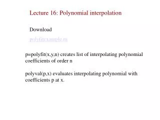
5. Determining Coefficients • Since polynomial interpolation provides as many basis functions as there are data points (n), the polynomial coefficients can be found exactly using linear algebra • For n data points, there is one and only one polynomial of order (n-1) that passes through all the points • MATLAB’s built in polyfit and polyval commands can also be used - all that is required is making sure the order of the fit for n data points is n-1

6. Polynomial Interpolation Problems • One problem that can occur with solving for the coefficients of a polynomial is that the system to be inverted is in the form: • Matrices such as that on the left are known as Vandermonde matrices, and they are very ill-conditioned - meaning their solutions are very sensitive to round-off errors • The issue can be minimized by scaling and shifting the data

7. Newton Interpolating Polynomials • Another way to express a polynomial interpolation is to use Newton’s interpolating polynomial • The differences between a simple polynomial and Newton’s interpolating polynomial for first and second order interpolations are:

8. Newton Interpolating Polynomials (1/3) • The first-order Newton interpolating polynomial may be obtained from linear interpolation and similar triangles, as shown • The resulting formula based on known points x1 and x2 and the values of the dependent function at those points is: designate a first-order polynomial

9. Linear Interpolation: An Example Example 17.2 The smaller the interval between the data points, the better the approximation.

10. Newton Interpolating Polynomials (2/3) • The second-order Newton interpolating polynomial introduces some curvature to the line connecting the points, but still goes through the first two points • The resulting formula based on known points x1, x2, and x3 and the values of the dependent function at those points is:

11. Quadratic Interpolation: An Example Example 17.3

12. Newton Interpolating Polynomials (3/3) • In general, an (n-1)th Newton interpolating polynomial has all the terms of the (n-2)th polynomial plus one extra • The general formula is: where and the f[…] represent divided differences

13. Divided Differences • Divided difference are calculated as follows: • Divided differences are calculated using divided difference of a smaller number of terms:

14. MATLAB Implementation

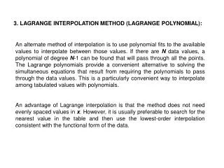
15. Lagrange Interpolating Polynomials (1/3) • Another method that uses shifted values to express an interpolating polynomial is the Lagrange interpolating polynomial • The differences between a simply polynomial and Lagrange interpolating polynomials for first and second order polynomials is: • where the are weighting coefficients of the jth polynomial, which are functions of x

16. Lagrange Interpolating Polynomials (2/3) • The first-order Lagrange interpolating polynomial may be obtained from a weighted combination of two linear interpolations, as shown • The resulting formula based on known points x1 and x2 and the values of the dependent function at those points is:

17. Lagrange Interpolating Polynomials (3/3) • In general, the Lagrange polynomial interpolation for n points is: • where is given by:

18. Lagrange Interpolating Polynomial: An Example

19. MATLAB Implementation

20. Inverse Interpolation (1/2) • Interpolation general means finding some value f(x) for some x that is between given independent data points • Sometimes, it will be useful to find the x for which f(x) is a certain value - this is inverse interpolation Some adjacent points of f(x) are bunched together and others spread out widely. This would lead to oscillations in the resulting polynomial.

21. Inverse Interpolation (2/2) • Rather than finding an interpolation of x as a function of f(x), it may be useful to find an equation for f(x) as a function of x using interpolation and then solve the corresponding roots problem:f(x)-fdesired=0 for x

22. Extrapolation • Extrapolation is the process of estimating a value of f(x) that lies outside the range of the known base points x1, x2, …, xn • Extrapolation represents a step into the unknown, and extreme care should be exercised when extrapolating!

23. Extrapolation Hazards • The following shows the results of extrapolating a seventh-order polynomial which is derived from the first 8 points (1920 to 1990) of the USA population data set:

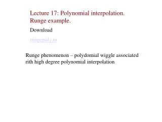
24. Oscillations • Higher-order polynomials can not only lead to round-off errors due to ill-conditioning, but can also introduce oscillations to an interpolation or fit where they should not be • In the figures below, the dashed line represents an function, the circles represent samples of the function, and the solid line represents the results of a polynomial interpolation: