Download
1 / 26
260 likes | 353 Vues
Land surface phenology versus traditional observations. Márta Hunkár (1) , Ildikó Szenyán , Enikő Vincze, Zoltán Dunkel (2) Tibor Szerdahelyi (3) (1) Georgikon Faculty University of Pannonia; hunkar@ georgikon.hu

E N D
Land surface phenology versus traditional observations Márta Hunkár (1) , Ildikó Szenyán , Enikő Vincze, Zoltán Dunkel (2) Tibor Szerdahelyi (3) (1) Georgikon Faculty University of Pannonia; hunkar@georgikon.hu (2) HungarianMeteorological Service; szenyan.i@met.hu; vincze.e@met.hu; dunkel.z@met.hu (3) Szent István University Institute of Botany and Ecophysiolgy; Szerdahelyi.Tibor@mkk.szie.hu EMS&ECAM 2013 09-13 Sept. Reading UK
EMS&ECAM 2013 09-13 Sept. Reading UK Outline • Aims • Material • Methods • Results • Conclusions
EMS&ECAM 2013 09-13 Sept. Reading UK Aims of our study • Retrieve land surface phenological data from satellite observations • Comparing traditional phenological observation data with land surface phenological data
EMS&ECAM 2013 09-13 Sept. Reading UK Introduction Traditional phenology Land surface phenology • Dates of phenological phases • Based on visual observation • Species-level • Local • Dates of critical values of vegetation indices • Based on satellite observation • Ecosystem level • Areal
EMS&ECAM 2013 09-13 Sept. Reading UK Material • Sample area: Iklad (5 km x 5 km) covered by different agricultural and native plants 47,6802 o N; 19,4217 o E 47,6802 o N; 19,4836 o E 47,6385 o N; 19,4063 o E 47,6385 o N; 19,4681 o E
from MODIS placed at Terra and Aqua satellites. Data are provided byNASA Land Processes Distributed Active Archive Center (NASA, LP DAAC, 2011). The MODIS Vegetation Index algorithm operates on a per-pixel basis and relies on multiple observations over a 16-day period to generate a composited Vegetation Index both from Terra and Aqua. We used high resolution (250m x250m pixels) composite data with 8 day frequency for the last ten years (2003-2012) on a sample area with the size of where L is a soil adjustment factor, and C1 and C2are coefficients used to correct aerosol scattering in the red band by the use of the blue band. The ρblue, ρred, and ρnirrepresent reflectance at the blue (0.45-0.52μm), red (0.6-0.7μm), and near-infrared (NIR) wavelengths (0.7-1.1μm), respectively. In general, G=2.5, C1=6.0, C2=7.5, and L=1. where L is a soil adjustment factor, and C1 and C2are coefficients used to correct aerosol scattering in the red band by the use of the blue band. The ρblue, ρred, and ρnirrepresent reflectance at the blue (0.45-0.52μm), red (0.6-0.7μm), and near-infrared (NIR) wavelengths (0.7-1.1μm), respectively. In general, G=2.5, C1=6.0, C2=7.5, and L=1. where L is a soil adjustment factor, and C1 and C2are coefficients used to correct aerosol scattering in the red band by the use of the blue band. The ρblue, ρred, and ρnirrepresent reflectance at the blue (0.45-0.52μm), red (0.6-0.7μm), and near-infrared (NIR) wavelengths (0.7-1.1μm), respectively. In general, G=2.5, C1=6.0, C2=7.5, and L=1. EMS&ECAM 2013 09-13 Sept. Reading UK Material • Satellite data: • Enhanced Vegetation Index (EVI) from MODIS placed at Terra and Aqua satellites (NASA, LP DAAC, 2011) The MODIS Vegetation Index algorithm operates on a per-pixel basis and relies on multiple observations over a 16-day period to generate a composited Vegetation Index both from Terra and Aquasatellitesoverlapped with 8 days. We got high resolution (250m x250m pixels) composite data with 8 day frequency for the last ten years (2003-2012) . The average EVI of that 400 pixels was used to characterise land surface vegetation.
EMS&ECAM 2013 09-13 Sept. Reading UK Material • where L is a soil adjustment factor, and C1 and C2are coefficients used to correct aerosol scattering in the red band by the use of the blue band. The ρblue, ρred, and ρnirrepresent reflectance at the blue (0.45-0.52μm), red (0.6-0.7μm), and near-infrared (NIR) wavelengths (0.7-1.1μm), respectively. In general, G=2.5, C1=6.0, C2=7.5, and L=1.
EMS&ECAM 2013 09-13 Sept. Reading UK Material • Traditionalobservations • Within the same sample areain 2011 and 2012 • Plants: • locust (Robinia pseudacacia); • poplar (Populus spp); • sessile oak, (Quercus petraea); • winter wheat (Triticum aestivum); • maize (Zea Mays); • sunflower (Helianthus annuus); native plants agricultural plants
EMS&ECAM 2013 09-13 Sept. Reading UK Material • The site of the traditional observations were identified by pixel-level (250m x 250m) • The EVI values of those pixels were analysed.
EMS&ECAM 2013 09-13 Sept. Reading UK Methods • Spatial average of high resolution EVI data is used to characterize of the vegetation dynamics. • Temporal variation in EVI data are modelled using piecewise sigmoid models. Each growth cycle is modelled using two sigmoid functions: one for the growth phase, one for the senescence phase.
EMS&ECAM 2013 09-13 Sept. Reading UK • To identify the land surface phenological transition dates, the rate of change in the curvature of the fitted logistic models is used for each year. • Specifically, transition dates correspond to the times at which the rate of change in curvature in the EVI data exhibits local minima or maximums.
EMS&ECAM 2013 09-13 Sept. Reading UK Time course of the spatial average EVI values for the sample area
EMS&ECAM 2013 09-13 Sept. Reading UK rate of change in the curvature of the fitted logistic models Increasing period of EVI
EMS&ECAM 2013 09-13 Sept. Reading UK Causes of shifting?
EMS&ECAM 2013 09-13 Sept. Reading UK • The corresponding phenological transition dates are defined as • the onset of greenness increase (F1), • the onset of greenness maximum (F2), • the onset of greenness decrease (F3), and • the onset of greenness minimum (F4).
EMS&ECAM 2013 09-13 Sept. Reading UK Trends of the length of the growing season(F4-F1, F3-F2)
EMS&ECAM 2013 09-13 Sept. Reading UK Traditional observations of trees
EMS&ECAM 2013 09-13 Sept. Reading UK Traditional observations of trees
EMS&ECAM 2013 09-13 Sept. Reading UK EVI values on pixel level
EMS&ECAM 2013 09-13 Sept. Reading UK EVI values on pixel level
EMS&ECAM 2013 09-13 Sept. Reading UK Traditional observation of agricultural plants
EMS&ECAM 2013 09-13 Sept. Reading UK Traditional observation of agricultural plants
EMS&ECAM 2013 09-13 Sept. Reading UK EVI values on pixel level Heading or flowering Harvest
EMS&ECAM 2013 09-13 Sept. Reading UK EVI values on pixel level
EMS&ECAM 2013 09-13 Sept. Reading UK Conclusions • Landscape phenology based on EVI is suitable to evaluate the vegetation dynamic of the season. • Traditional phenology is more sophisticated but it is difficult to integrate. • EVI values for native plants (trees) can be modeled by logistic curves. • Flowering time relating to EVI is plant specific • EVI values for agricultural plants show different shape (not logistic). • The maximum EVI is around flowering and then the decreasing phase has rather convex curvature.
EMS&ECAM 2013 09-13 Sept. Reading UK Thank you for your attention!