Parametric Statistical Inference

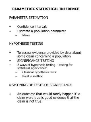
1. Parametric Statistical Inference Instructor: Ron S. Kenett Email: ron@kpa.co.il Course Website: www.kpa.co.il/biostat Course textbook: MODERN INDUSTRIAL STATISTICS, Kenett and Zacks, Duxbury Press, 1998 (c) 2001, Ron S. Kenett, Ph.D.

2. Course Syllabus • Understanding Variability • Variability in Several Dimensions • Basic Models of Probability • Sampling for Estimation of Population Quantities • Parametric Statistical Inference • Computer Intensive Techniques • Multiple Linear Regression • Statistical Process Control • Design of Experiments (c) 2001, Ron S. Kenett, Ph.D.

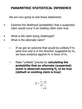
3. Definitions • Null Hypotheses • H0: Put here what is typical of the population, a term that characterizes “business as usual” where nothing out of the ordinary occurs. • Alternative Hypotheses • H1: Put here what is the challenge, the view of some characteristic of the population that, if it were true, would trigger some new action, some change in procedures that had previously defined “business as usual.” (c) 2001, Ron S. Kenett, Ph.D.

4. The Logic of Hypothesis Testing • A new claim is asserted that challenges existing thoughts about a population characteristic. • Suggestion: Form the alternative hypothesis first, since it embodies the challenge. • Step 1. A claim is made. (c) 2001, Ron S. Kenett, Ph.D.

5. The Logic of Hypothesis Testing • Step 2. How much error are you willing to accept? • Select the maximum acceptable error, a. The decision maker must elect how much error he/she is willing to accept in making an inference about the population. The significance level of the test is the maximum probability that the null hypothesis will be rejected incorrectly, a Type I error. (c) 2001, Ron S. Kenett, Ph.D.

6. The Logic of Hypothesis Testing • Assume the null hypothesis is true. This is a very powerful statement. The test is always referenced to the null hypothesis. Form the rejection region, the areas in which the decision maker is willing to reject the presumption of the null hypothesis. • Step 3. If the null hypothesis were true, what would you expect to see? (c) 2001, Ron S. Kenett, Ph.D.

7. The Logic of Hypothesis Testing • Step 4. What did you actually see? • Compute the sample statistic. The sample provides a set of data that serves as a window to the population. The decision maker computes the sample statistic and calculates how far the sample statistic differs from the presumed distribution that is established by the null hypothesis. (c) 2001, Ron S. Kenett, Ph.D.

8. The Logic of Hypothesis Testing • Step 5. Make the decision. • The decision is a conclusion supported by evidence. The decision maker will: • reject the null hypothesis if the sample evidence is so strong, the sample statistic so unlikely, that the decision maker is convinced H1 must be true. • fail to reject the null hypothesis if the sample statistic falls in the nonrejection region. In this case, the decision maker is not concluding the null hypothesis is true, only that there is insufficient evidence to dispute it based on this sample. (c) 2001, Ron S. Kenett, Ph.D.

9. The Logic of Hypothesis Testing • Step 6. What are the implications of the decision for future actions? • State what the decision means in terms of the research program. The decision maker must draw out the implications of the decision. Is there some action triggered, some change implied? What recommendations might be extended for future attempts to test similar hypotheses? (c) 2001, Ron S. Kenett, Ph.D.

10. Two Types of Errors • Type I Error: • Saying you reject H0 when it really is true. • Rejecting a true H0. • Type II Error: • Saying you do not reject H0 when it really is false. • Failing to reject a false H0. (c) 2001, Ron S. Kenett, Ph.D.

11. What are acceptable error levels? • Decision makers frequently use a 5% significance level. • Use a = 0.05. • An a-error means that we will decide to adjust the machine when it does not need adjustment. • This means, in the case of the robot welder, if the machine is running properly, there is only a 0.05 probability of our making the mistake of concluding that the robot requires adjustment when it really does not. (c) 2001, Ron S. Kenett, Ph.D.

12. Three Types of Tests • Nondirectional, two-tail test: • H1: pop parameter n.e. value • Directional, right-tail test: • H1: pop parameter > value • Directional, left-tail test: • H1: pop parameter < value Always put hypotheses in terms of population parameters and have H0: pop parameter = value (c) 2001, Ron S. Kenett, Ph.D.

13. Two tailed test • H0: pop parameter = value • H1: pop parameter n.e. value (c) 2001, Ron S. Kenett, Ph.D.

14. Right tailed test • H0: pop parameter = value • H1: pop parameter > value (c) 2001, Ron S. Kenett, Ph.D.

15. Left tailed test • H0: pop parameter = value • H1: pop parameter < value (c) 2001, Ron S. Kenett, Ph.D.

16. Reality Ho H1 TypeI Error H1 OK Decision TypeII Error OK Ho (c) 2001, Ron S. Kenett, Ph.D.

17. What Test to Apply? Ask the following questions: • Are the data the result of a measurement (a continuous variable) or a count (a discrete variable)? • Is s known? • What shape is the distribution of the population parameter? • What is the sample size? (c) 2001, Ron S. Kenett, Ph.D.

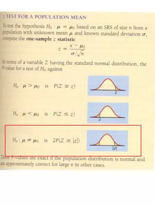
18. m x – 0 = z s n Test of µ, s Known, Population Normally Distributed • Test Statistic: • where • is the sample statistic. • µ0 is the value identified in the null hypothesis. • s is known. • n is the sample size. (c) 2001, Ron S. Kenett, Ph.D.

19. m x – 0 = z s n Test of µ, s Known, Population Not Normally Distributed • If n> 30, Test Statistic: • If n < 30, use a distribution-free test. (c) 2001, Ron S. Kenett, Ph.D.

20. 0 = t s n x Test of µ, s Unknown, Population Normally Distributed • Test Statistic: • where • is the sample statistic. • µ0 is the value identified in the null hypothesis. • s is unknown. • n is the sample size • degrees of freedom on t are n– 1. m x – (c) 2001, Ron S. Kenett, Ph.D.

21. Test of µ, s Unknown, Population Not Normally Distributed • If n> 30, Test Statistic: • If n < 30, use a distribution-free test. (c) 2001, Ron S. Kenett, Ph.D.

22. Test of p, Sample Sufficiently Large • If both n p> 5 and n(1 –p) > 5, Test Statistic: • where p = sample proportion • p0 is the value identified in the null hypothesis. • n is the sample size. (c) 2001, Ron S. Kenett, Ph.D.

23. Test of p, Sample Not Sufficiently Large • If either n p< 5 or n(1 –p) < 5, convert the proportion to the underlying binomial distribution. • Note there is no t-test on a population proportion. (c) 2001, Ron S. Kenett, Ph.D.

24. Observed Significance Levels • A p-Value is: • the exact level of significance of the test statistic. • the smallest value a can be and still allow us to reject the null hypothesis. • the amount of area left in the tail beyond the test statistic for a one-tailed hypothesis test or • twice the amount of area left in the tail beyond the test statistic for a two-tailed test. • the probability of getting a test statistic from another sample that is at least as far from the hypothesized mean as this sample statistic is. (c) 2001, Ron S. Kenett, Ph.D.

25. Observed Significance Levels • A p-Value is: • the exact level of significance of the test statistic. • the smallest value a can be and still allow us to reject the null hypothesis. • the amount of area left in the tail beyond the test statistic for a one-tailed hypothesis test or • twice the amount of area left in the tail beyond the test statistic for a two-tailed test. • the probability of getting a test statistic from another sample that is at least as far from the hypothesized mean as this sample statistic is. (c) 2001, Ron S. Kenett, Ph.D.

26. Several Samples • Independent Samples: • Testing a company’s claim that its peanut butter contains less fat than that produced by a competitor. • Dependent Samples: • Testing the relative fuel efficiency of 10 trucks that run the same route twice, once with the current air filter installed and once with the new filter. (c) 2001, Ron S. Kenett, Ph.D.

27. Test of (µ1–µ2), s1 = s2, Populations Normal m m [ x – x ] – [ – ] 1 2 1 2 = t ! ! 1 1 2 ! ! + s ! ! p n n ! ! 1 2 ! ! ! ! ! ! 2 2 + ( n – 1 ) s ( n – 1 ) s 2 1 1 2 2 = where s p + n n – 2 1 2 • Test Statistic • where degrees of freedom on t = n1 + n2– 2 (c) 2001, Ron S. Kenett, Ph.D.

28. Example:Comparing Two populations • H0: pop1 = pop2 • H1: pop1 n.e. pop2 Hypothesis Assumption Test Statistic The mean of population 1 is equal to the mean of population 2 (1) Both distributions are normal (2) s1 = s2 t distribution with df = n1+ n2-2 (c) 2001, Ron S. Kenett, Ph.D.

29. Example:Comparing Two populations Rejection Region Rejection Region t distribution with df = n1+ n2-2 (c) 2001, Ron S. Kenett, Ph.D.

30. Test of (µ1–µ2), s1 n.e. s2, Populations Normal, large n m m [ x – x ] – [ – ] 1 2 1 2 0 = z 2 2 s s 1 2 + n n 1 2 • Test Statistic • with s12 and s22 as estimates for s12 and s22 (c) 2001, Ron S. Kenett, Ph.D.

31. Test of Dependent Samples(µ1–µ2) = µd d = t s d n • Test Statistic • where d = (x1–x2) = Sd/n, the average difference n = the number of pairs of observations sd = the standard deviation of d df = n– 1 (c) 2001, Ron S. Kenett, Ph.D.

32. n p + n p 1 1 2 2 p = n + n 1 2 Test of (p1–p2), where n1p1>5, n1(1–p1)>5, n2p2>5, and n2 (1–p2 )>5 • Test Statistic • where p1 = observed proportion, sample 1 p2 = observed proportion, sample 2 n1 = sample size, sample 1 n2 = sample size , sample 2 (c) 2001, Ron S. Kenett, Ph.D.

33. Test of Equal Variances • Pooled-variances t-test assumes the two population variances are equal. • The F-test can be used to test that assumption. • The F-distribution is the sampling distribution of s12/s22 that would result if two samples were repeatedly drawn from a single normally distributed population. (c) 2001, Ron S. Kenett, Ph.D.

34. Test of s12 = s22 2 2 s s 1 2 = F or 2 2 s s 2 1 • If s12 = s22 , then s12/s22 = 1. So the hypotheses can be worded either way. • Test Statistic: whichever is larger • The critical value of the F will be F(a/2, n1, n2) • where a = the specified level of significance n1 = (n– 1), where n is the size of the sample with the larger variance n2 = (n– 1), where n is the size of the sample with the smaller variance (c) 2001, Ron S. Kenett, Ph.D.

35. 1 1 ! ! 2 ± ׳ + ! ! ( x – x ) t s a ! ! p 1 2 ! ! 2 n n ! ! 1 2 ! ! ! ! 2 2 s s 1 2 ± ׳ + ( x – x ) z a 1 2 n n 2 1 2 Confidence Interval for (µ1–µ2) • The (1 –a)% confidence interval for the difference in two means: • Equal variances, populations normal • Unequal variances, large samples (c) 2001, Ron S. Kenett, Ph.D.

36. Confidence Interval for (p1–p2) p ( 1 – p ) p ( 1 – p ) 1 1 2 2 ± ׳ + ( p – p ) z a 1 2 n n 2 1 2 • The (1 –a)% confidence interval for the difference in two proportions: • when sample sizes are sufficiently large. (c) 2001, Ron S. Kenett, Ph.D.

37. t distribution with df = n1+ n2-2 F distribution with df2 = n1-1 and df2 = n2-1 Z - Normal distribution Summary Hypothesis Assumption Test Statistic The mean of population 1 is equal to the mean of population 2 (1) Both distributions are normal (2) s1 = s2 The standard deviation of population 1 is equal to the standard deviation of population 2 Both distributions are normal The proportion of error in population 1 is equal to the proportion of errors in population 2 n1p1 and n2p2> 5 (approximation by normal distribution) (c) 2001, Ron S. Kenett, Ph.D.