Experiment
Experiment. Here is an experiment that demonstrates Ferson’s point (see Ferson, Sarkissian and Simin, Journal of Financial Markets 2 (1), 49-68, February 1999)

Experiment
E N D
Presentation Transcript
Experiment • Here is an experiment that demonstrates Ferson’s point (see Ferson, Sarkissian and Simin, Journal of Financial Markets 2 (1), 49-68, February 1999) • In this experiment, returns are generated such that cross-sectional differences are entirely due to non-risk reasons. However loadings on the spread portfolio “explain” these differences, so there appears to be a common risk factor
Set-up • We want to generate returns that: • Match the (unconditional) cross-sectional average • Have cross-sectional differences that are associated with some non-risk attribute • Have time-varying predictable properties • Have co-movement in returns
Return simulation • Sort stocks into 100 portfolios based on first 2 letters of the firm’s name • Introduce systematic behavior into returns through simulated excess return rSIM rSIM = μACT + δ0 + δ1’zt-1 + εSIM
Siimulated return components • Constant (grand mean of excess return across portfolios) μACT • Cross-sectional difference δ0 • Center at zero • Return difference between highest and lowest = actual value premium, spread equally across portfolios
Simulated return components • Predictable time variation • Instruments zt-1 • 3-month T-bill • Dividend yield on S&P500 • Expressed as deviations from mean • Coefficients δ1 • Regress HML on zt-1 • Centering at zero, spread out each coefficient uniformly across 100 portfolios • Rescale to destroy uniformity in coefficients
Simulated return components • Residual return • For each portfolio p regress its time series of actual excess return on zt-1, get eP • Regress time series of S&P500 excess returns on δ1’zt-1, get eM • Regress eP on eM, collect slope coefficients in b • Let V(ε) = bb’ + σ2IN • Transform eP such that their variances = V(ε)
Risk versus characteristics • Researcher looks at returns on the alphabet-sorted portfolios • Builds factor-mimicking portfolio AMZ that goes long low-alphabet order (‘A’) firms and goes short high-alphabet order (‘Z’) firms • Does 2-pass CSR rsimpt = γ0 + γ1βpM + γ2βpAMZ + γ3 Wpt + ξpt