Frequency Distribution, Cross-Tabulation, and Hypothesis Testing
Frequency Distribution, Cross-Tabulation, and Hypothesis Testing. Internet Usage Data. Table 15.1. Respondent Sex Familiarity Internet Attitude Toward Usage of Internet

Frequency Distribution, Cross-Tabulation, and Hypothesis Testing
E N D
Presentation Transcript
Frequency Distribution, Cross-Tabulation, and Hypothesis Testing
Internet Usage Data Table 15.1 Respondent Sex Familiarity Internet Attitude Toward Usage of Internet NumberUsageInternet Technology Shopping Banking 1 1.00 7.00 14.00 7.00 6.00 1.00 1.00 2 2.00 2.00 2.00 3.00 3.00 2.00 2.00 3 2.00 3.00 3.00 4.00 3.00 1.00 2.00 4 2.00 3.00 3.00 7.00 5.00 1.00 2.00 5 1.00 7.00 13.00 7.00 7.00 1.00 1.00 6 2.00 4.00 6.00 5.00 4.00 1.00 2.00 7 2.00 2.00 2.00 4.00 5.00 2.00 2.00 8 2.00 3.00 6.00 5.00 4.00 2.00 2.00 9 2.00 3.00 6.00 6.00 4.00 1.00 2.00 10 1.00 9.00 15.00 7.00 6.00 1.00 2.00 11 2.00 4.00 3.00 4.00 3.00 2.00 2.00 12 2.00 5.00 4.00 6.00 4.00 2.00 2.00 13 1.00 6.00 9.00 6.00 5.00 2.00 1.00 14 1.00 6.00 8.00 3.00 2.00 2.00 2.00 15 1.00 6.00 5.00 5.00 4.00 1.00 2.00 16 2.00 4.00 3.00 4.00 3.00 2.00 2.00 17 1.00 6.00 9.00 5.00 3.00 1.00 1.00 18 1.00 4.00 4.00 5.00 4.00 1.00 2.00 19 1.00 7.00 14.00 6.00 6.00 1.00 1.00 20 2.00 6.00 6.00 6.00 4.00 2.00 2.00 21 1.00 6.00 9.00 4.00 2.00 2.00 2.00 22 1.00 5.00 5.00 5.00 4.00 2.00 1.00 23 2.00 3.00 2.00 4.00 2.00 2.00 2.00 24 1.00 7.00 15.00 6.00 6.00 1.00 1.00 25 2.00 6.00 6.00 5.00 3.00 1.00 2.00 26 1.00 6.00 13.00 6.00 6.00 1.00 1.00 27 2.00 5.00 4.00 5.00 5.00 1.00 1.00 28 2.00 4.00 2.00 3.00 2.00 2.00 2.00 29 1.00 4.00 4.00 5.00 3.00 1.00 2.00 30 1.00 3.00 3.00 7.00 5.00 1.00 2.00
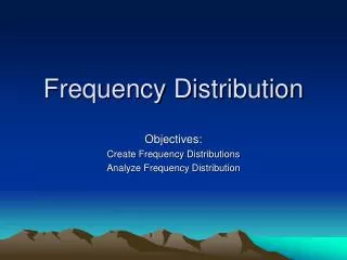
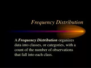
Frequency Distribution • In a frequency distribution, one variable is considered at a time. • A frequency distribution for a variable produces a table of frequency counts, percentages, and cumulative percentages for all the values associated with that variable.
Frequency Distribution of Familiaritywith the Internet Table 15.2
Frequency Histogram Figure 15.1 8 7 6 5 Frequency 4 3 2 1 0 2 3 4 7 6 5 Familiarity
Statistics Associated with Frequency DistributionMeasures of Shape • Skewness. The tendency of the deviations from the mean to be larger in one direction than in the other. It can be thought of as the tendency for one tail of the distribution to be heavier than the other. • Kurtosis is a measure of the relative peakedness or flatness of the curve defined by the frequency distribution. The kurtosis of a normal distribution is zero. If the kurtosis is positive, then the distribution is more peaked than a normal distribution. A negative value means that the distribution is flatter than a normal distribution.
Skewness of a Distribution Figure 15.2 Symmetric Distribution Skewed Distribution Mean Median Mode (a) Mean Median Mode (b)
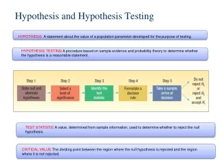
A General Procedure for Hypothesis TestingFormulate the Hypothesis • A null hypothesis is a statement of the status quo, one of no difference or no effect. If the null hypothesis is not rejected, no changes will be made. • An alternative hypothesis is one in which some difference or effect is expected. Accepting the alternative hypothesis will lead to changes in opinions or actions. • The null hypothesis refers to a specified value of the population parameter (e.g., ), not a sample statistic (e.g., ).
H : p = 0 . 4 0 0 H 1 A General Procedure for Hypothesis TestingFormulate the Hypothesis • A null hypothesis may be rejected, but it can never be accepted based on a single test. In classical hypothesis testing, there is no way to determine whether the null hypothesis is true. • In marketing research, the null hypothesis is formulated in such a way that its rejection leads to the acceptance of the desired conclusion. The alternative hypothesis represents the conclusion for which evidence is sought. : p > 0 . 40
H 1 A General Procedure for Hypothesis TestingFormulate the Hypothesis • The test of the null hypothesis is a one-tailed test, because the alternative hypothesis is expressed directionally. If that is not the case, then a two-tailed test would be required, and the hypotheses would be expressed as: p H : = 0 . 4 0 0 : p ¹ 0 . 4 0
A General Procedure for Hypothesis TestingChoose a Level of Significance Type I Error • Type Ierror occurs when the sample results lead to the rejection of the null hypothesis when it is in fact true. • The probability of type I error ( ) is also called the level of significance. Type II Error • Type II error occurs when, based on the sample results, the null hypothesis is not rejected when it is in fact false. • The probability of type II error is denoted by . • Unlike , which is specified by the researcher, the magnitude of depends on the actual value of the population parameter (proportion).
A General Procedure for Hypothesis TestingChoose a Level of Significance Power of a Test • The power of a test is the probability (1 - ) of rejecting the null hypothesis when it is false and should be rejected. • Although is unknown, it is related to . An extremely low value of (e.g., = 0.001) will result in intolerably high errors. • So it is necessary to balance the two types of errors.
A General Procedure for Hypothesis TestingBusiness Research Conclusion • The conclusion reached by hypothesis testing must be expressed in terms of the marketing research problem. • For example, if Ho is rejected, we conclude that there is evidence that the proportion of Internet users who shop via the Internet is significantly greater than 0.40. Hence, the recommendation to the department store would be to introduce the new Internet shopping service.
Hypothesis Tests Tests of Differences Tests of Association Median/ Rankings Proportions Means Distributions A Broad Classification of Hypothesis Tests Figure 15.6
Cross-Tabulation • While a frequency distribution describes one variable at a time, a cross-tabulation describes two or more variables simultaneously. • Cross-tabulation results in tables that reflect the joint distribution of two or more variables with a limited number of categories or distinct values, e.g., Table 15.3.
Gender and Internet Usage Table 15.3
Two Variables Cross-Tabulation • Since two variables have been cross classified, percentages could be computed either columnwise, based on column totals (Table 15.4), or rowwise, based on row totals (Table 15.5). • The general rule is to compute the percentages in the direction of the independent variable, across the dependent variable. The correct way of calculating percentages is as shown in Table 15.4.
Internet Usage by Gender Table 15.4
Gender by Internet Usage Table 15.5
Statistics Associated with Cross-TabulationChi-Square • To determine whether a systematic association exists, the probability of obtaining a value of chi-square as large or larger than the one calculated from the cross-tabulation is estimated. • An important characteristic of the chi-square statistic is the number of degrees of freedom (df) associated with it. That is, df = (r - 1) x (c -1). • The null hypothesis (H0) of no association between the two variables will be rejected only when the calculated value of the test statistic is greater than the critical value of the chi-square distribution with the appropriate degrees of freedom, as shown in Figure 15.8.
Chi-square Distribution Figure 15.8 Do Not Reject H0 Reject H0 2 Critical Value
Statistics Associated with Cross-TabulationPhi Coefficient • The phi coefficient ( ) is used as a measure of the strength of association in the special case of a table with two rows and two columns (a 2 x 2 table). • The phi coefficient is proportional to the square root of the chi-square statistic • It takes the value of 0 when there is no association, which would be indicated by a chi-square value of 0 as well. When the variables are perfectly associated, phi assumes the value of 1 and all the observations fall just on the main or minor diagonal.
Statistics Associated with Cross-TabulationContingency Coefficient • While the phi coefficient is specific to a 2 x 2 table, the contingency coefficient(C) can be used to assess the strength of association in a table of any size. • The contingency coefficient varies between 0 and 1. • The maximum value of the contingency coefficient depends on the size of the table (number of rows and number of columns). For this reason, it should be used only to compare tables of the same size.
Statistics Associated with Cross-TabulationCramer’s V • Cramer's V is a modified version of the phi correlation coefficient, , and is used in tables larger than 2 x 2. or
Statistics Associated with Cross-TabulationLambda Coefficient • Asymmetric lambda measures the percentage improvement in predicting the value of the dependent variable, given the value of the independent variable. • Lambda also varies between 0 and 1. A value of 0 means no improvement in prediction. A value of 1 indicates that the prediction can be made without error. This happens when each independent variable category is associated with a single category of the dependent variable. • Asymmetric lambda is computed for each of the variables (treating it as the dependent variable). • A symmetric lambda is also computed, which is a kind of average of the two asymmetric values. The symmetric lambda does not make an assumption about which variable is dependent. It measures the overall improvement when prediction is done in both directions.
Statistics Associated with Cross-TabulationOther Statistics • Other statistics like taub, tauc, and gamma are available to measure association between two ordinal-level variables. Both tau b and tau c adjust for ties. • Taub is the most appropriate with square tables in which the number of rows and the number of columns are equal. Its value varies between +1 and -1. • For a rectangular table in which the number of rows is different than the number of columns, tauc should be used. • Gamma does not make an adjustment for either ties or table size. Gamma also varies between +1 and -1 and generally has a higher numerical value than tau b or tauc.
Cross-Tabulation in Practice While conducting cross-tabulation analysis in practice, it is useful to proceed along the following steps. • Test the null hypothesis that there is no association between the variables using the chi-square statistic. If you fail to reject the null hypothesis, then there is no relationship. • If H0 is rejected, then determine the strength of the association using an appropriate statistic (phi-coefficient, contingency coefficient, Cramer's V, lambda coefficient, or other statistics), as discussed earlier. • If H0 is rejected, interpret the pattern of the relationship by computing the percentages in the direction of the independent variable, across the dependent variable. • If the variables are treated as ordinal rather than nominal, use taub, tau c, or Gamma as the test statistic. If H0 is rejected, then determine the strength of the association using the magnitude, and the direction of the relationship using the sign of the test statistic.
Hypothesis Testing Related to Differences • Parametric tests assume that the variables of interest are measured on at least an interval scale. • Nonparametric tests assume that the variables are measured on a nominal or ordinal scale. • These tests can be further classified based on whether one or two or more samples are involved. • The samples are independent if they are drawn randomly from different populations. For the purpose of analysis, data pertaining to different groups of respondents, e.g., males and females, are generally treated as independent samples. • The samples are paired when the data for the two samples relate to the same group of respondents.
SPSS Windows • The main program in SPSS is FREQUENCIES. It produces a table of frequency counts, percentages, and cumulative percentages for the values of each variable. It gives all of the associated statistics. • If the data are interval scaled and only the summary statistics are desired, the DESCRIPTIVES procedure can be used. • The EXPLORE procedure produces summary statistics and graphical displays, either for all of the cases or separately for groups of cases. Mean, median, variance, standard deviation, minimum, maximum, and range are some of the statistics that can be calculated.
SPSS Windows To select these procedures click: Analyze>Descriptive Statistics>Frequencies Analyze>Descriptive Statistics>Descriptives Analyze>Descriptive Statistics>Explore The major cross-tabulation program is CROSSTABS. This program will display the cross-classification tables and provide cell counts, row and column percentages, the chi-square test for significance, and all the measures of the strength of the association that have been discussed. To select these procedures click: Analyze>Descriptive Statistics>Crosstabs
SPSS Windows The major program for conducting parametric tests in SPSS is COMPARE MEANS. This program can be used to conduct t tests on one sample or independent or paired samples. To select these procedures using SPSS for Windows click: Analyze>Compare Means>Means … Analyze>Compare Means>One-Sample T Test … Analyze>Compare Means>Independent- Samples T Test … Analyze>Compare Means>Paired-Samples T Test …
SPSS Windows The nonparametric tests discussed in this chapter can be conducted using NONPARAMETRIC TESTS. To select these procedures using SPSS for Windows click: Analyze>Nonparametric Tests>Chi-Square … Analyze>Nonparametric Tests>Binomial … Analyze>Nonparametric Tests>Runs … Analyze>Nonparametric Tests>1-Sample K-S … Analyze>Nonparametric Tests>2 Independent Samples … Analyze>Nonparametric Tests>2 Related Samples …