Download
1 / 22
260 likes | 907 Vues
LECTURE 13 ANALYSIS OF COVARIANCE AND COVARIANCE INTERACTION. and ATI (Aptitude-Treatment Interaction). ANCOVA. ANCOVA model The simplest ANCOVA model includes a covariate C , an exogenous treatment variable X , and an outcome Y : y ij = y + i ij + c ij + e ij

E N D
LECTURE 13ANALYSIS OF COVARIANCE AND COVARIANCE INTERACTION and ATI (Aptitude-Treatment Interaction)
ANCOVA ANCOVA model The simplest ANCOVA model includes a covariate C, an exogenous treatment variable X, and an outcome Y: yij = y + iij + cij + eij This is a regression equation relating the exogenous variables to the endogenous outcome. In classical ANOVA terms, the model is written as yij = y + ii + (cij - c.. ) + eij In this formulation the grand mean y plays the same role as in ANOVA, the mean performance of all populations. The term ii is the effect of the treatment, and the term (cij - xi. ) is the regression effect of the covariate deviation from the covariate grand mean on the outcome. This equation can be rewritten as yij = (- C ) + ii + cij + eij
SOURCE df Sum of Squares Mean Square F Covariate 1 R2(cij – c..)2 SSc SSc/MSe Treatment…k-1 n(ŷi. – y..)2 SStreat / k-1 MStreat/MSe error n(k-1)-1 (ŷij - ŷi.)2 SSe / [n(k-1)-1] - total kn-1(ŷij – y..)2 SSy.c / (n-1) - Table 12.1: Analysis of Covariance table
SS SS y c SS c SS y SS Covariate SS Covariate e e ss , treat Type III SS SS e e ss treat b. Nonrandomized design a. Randomized design Fig. 12.4: Venn diagram for ANCOVA with covariate, k treatments and outcome
HLM Issues • Random Intercepts and Slopes: • Suppose we assume the regressions for the various groups are NOT based on fixed covariate values but that these are samples from the population (the real situation). Then the intercepts and slopes are not fixed but can vary randomly from sample to sample • This means that the covariate is a RANDOM factor, not a fixed factor; either or both intercept and slope could be random.
Random Covariate Parameters • Y = b0j + b1jXij + eij [student i in cluster j first level model] • b0j = g00 + g01Zj + u0j [intercept regression equation depends on cluster j second level value Z] • b1j = g10 + g11Zj + u1j [slope depends on cluster j second level value Z]
Random Covariate Parameters Example: students in a classroom: achievement Y is a function of expectation for mastery X Classrooms have a teacher-defined learning climate Z, and the level (intercept) of achievement Y depends on this climate as well as the relationship of achievement to expectation for mastery (slope)
Group 4 Random Covariate Parameters Group 3 b1j = g10 + g11Zj + u1j Y Random slopes Group 2 b0j = g00 + g01Zj + u0j Random intercepts Group 1 Covariate X
Mixed Models procedures • Fixed Effects ANOVA Table Source df MS F sig. • Random Effects Variance-Covariance Table Source Variance S.E. sig. Sources Covariance S.E. sig.
SAS approach procmixed noclprint covtest noitprint ; class cls ; model mnrat1=OVAG gen eth eth*gen gen*OVAG eth*OVAG gen*eth*OVAG /solution ddfm=bw ; random intercept OVAG/sub=cls type=un;
Covariance Parameter Estimates RANDOM EFFECTS Standard Z Cov Parm Subject Estimate Error Value Pr Z intercept UN(1,1) cls 0.1050 0.01486 7.06 <.0001 corr(i,s)UN(2,1) cls 0.02269 0.02523 0.90 0.3685 slope UN(2,2) cls 0.2211 0.08588 2.57 0.0050 Residual 0.3361 0.009478 35.46 <.0001 Type 3 Tests of Fixed Effects Num Den Effect DF DF F Value Pr > F OVAG 1 2650 435.46 <.0001 gen 1 152 18.43 <.0001 eth 1 164 18.99 <.0001 gen*eth 1 152 7.38 0.0074 OVAG*gen 1 2650 9.15 0.0025 OVAG*eth 1 2650 5.28 0.0217 OVAG*gen*eth 1 2650 0.03 0.8609