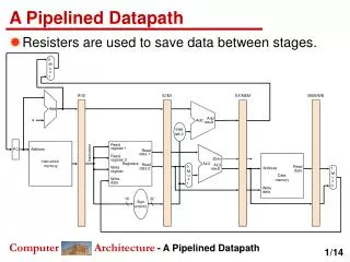
A Pipelined Processor

1. A Pipelined Processor Taken from Digital Design and Computer Architecture by Harris and Harris

2. Introduction • Microarchitecture: how to implement an architecture in hardware • Processor: • Datapath: functional blocks • Control: control signals

3. Microarchitecture • Multiple implementations for a single architecture: • Single-cycle • Each instruction executes in a single cycle • Multicycle • Each instruction is broken up into a series of shorter steps • Pipelined • Each instruction is broken up into a series of steps • Multiple instructions execute at once. • Microcode

4. Architectural State • Determines everything about a processor: • PC • 32 registers • Memory

5. Instruction Formats add sub or and … lw sw … beq bne …

6. State Elements: PC, 32 registers, and Memory

7. Single-Cycle Datapath: lw fetch • executing lw: lw (index reg) (destination reg) (immediate offset) example: lw $s3, 1($0) # read memory word 1 into $s3 rt <- DataMemory[rs+imm] • STEP 1: Fetch instruction

8. Single-Cycle Datapath: lw register read • STEP 2: Read source operands from register file

9. Single-Cycle Datapath: lw immediate • STEP 3: Sign-extend the immediate

10. Single-Cycle Datapath: lw address • STEP 4: Compute the memory address

11. Single-Cycle Datapath: lw memory read • STEP 5: Read data from memory and write it back to register file

12. Single-Cycle Datapath: lw PC increment • STEP 6: Determine the address of the next instruction

13. Single-Cycle Datapath: sw • sw: sw (index reg) (source reg) (immediate offset) • Write data in rt to memory

14. Single-Cycle Datapath: R-type instructions • example:rd <- rt + rs ; add $s0, $s1, $s2 • Read from rs and rt • Write ALUResult to register file • Write to rd (instead of rt)

15. Single-Cycle Datapath: beq • Determine whether values in rs and rt are equal beq $s0, $s1, target … target: # label • Calculate branch target address: BTA = (sign-extended immediate << 2) + (PC+4)

16. Complete Single-Cycle Processor

17. Review: Processor Performance Program Execution Time = (# instructions)(cycles/instruction)(seconds/cycle) = # instructions x CPI x TC

18. Single-Cycle Performance • TC is limited by the critical path (lw)

19. Single-Cycle Performance • Single-cycle critical path: • Tc = tpcq_PC + tmem + max(tRFread, tsext + tmux) + tALU + tmem + tmux + tRFsetup • In most implementations, limiting paths are: • memory, ALU, register file. • Tc = tpcq_PC + 2tmem + tRFread + tmux + tALU + tRFsetup

20. Single-Cycle Performance Example Tc =

21. Single-Cycle Performance Example Tc = tpcq_PC + 2tmem + tRFread + tmux + tALU + tRFsetup = [30 + 2(250) + 150 + 25 + 200 + 20] ps = 925 ps

22. Single-Cycle Performance Example • For a program with 100 billion instructions executing on a single-cycle MIPS processor, • Execution Time =

23. Single-Cycle Performance Example • For a program with 100 billion instructions executing on a single-cycle MIPS processor, • Execution Time = # instructions x CPI x TC • = (100 × 109)(1)(925 × 10-12 s) • = 92.5 seconds

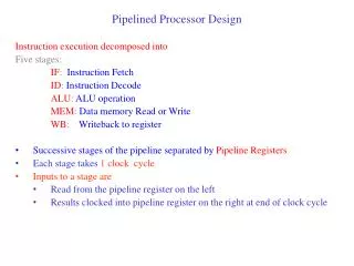
24. Pipelined Processor • Temporal parallelism • Divide single-cycle processor into 5 ROUGHLY EQUIVALENT stages: • Fetch • Decode • Execute • Memory • Writeback • Each stage includes one “slow step” • Add pipeline registers between stages • 5 stages => ~ 5 times faster! • All modern high-performance processors are pipelined.

25. Single-Cycle vs. Pipelined Performance The length of all pipeline stages is set by the slowest stage The instruction latency is 5 * 250 ps = 1250 ps

26. Pipelining Abstraction

27. Single-Cycle and Pipelined Datapath

28. Corrected Pipelined Datapath • WriteReg address must arrive at the same time as Result

29. Pipelined Control Same control unit as single-cycle processor Control delayed to proper pipeline stage

30. Pipeline Hazard • Occurs when an instruction depends on results from previous instruction that hasn’t completed. • Types of hazards: • Data hazard: register value not written back to register file yet • Control hazard: next instruction not decided yet (caused by branches)

31. Data Hazard

32. Handling Data Hazards Insert nops in code at compile time Rearrange code at compile time Forward data at run time Stall the processor at run time

33. Control Hazards • beq: • branch is not determined until the fourth stage of the pipeline • Instructions after the branch are fetched before branch occurs • These instructions must be flushed if the branch happens • Branch misprediction penalty • number of instruction flushed when branch is taken • May be reduced by determining branch earlier

34. Branch Prediction • Guess whether branch will be taken • Backward branches are usually taken (loops) • Perhaps consider history of whether branch was previously taken to improve the guess • Good prediction reduces the fraction of branches requiring a flush