Methodological summary of flood frequency analysis
340 likes | 598 Vues
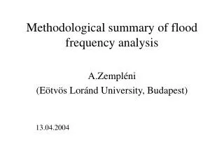
Methodological summary of flood frequency analysis. A.Zempl éni (Eötvös Loránd University, Budapest) 13 . 04 .200 4. Analysis of extreme values. Classical methods: based on annual maxima Peaks-over-threshold methods: utilize all floods higher than a given (high) threshold.

Methodological summary of flood frequency analysis
E N D
Presentation Transcript
Methodological summary of flood frequency analysis A.Zempléni (Eötvös Loránd University, Budapest) 13.04.2004
Analysis of extreme values • Classical methods: based on annual maxima • Peaks-over-threshold methods: utilize all floods higher than a given (high) threshold. • Multivariate modelling • Bayesian approach (dependence among parameters) • Joint behaviour of extremes
Extreme-value distributions Let be independent, identically distributed random variables. If we can find norming constants an, bn such that has a nondegenerate limit, then this limit is necessarily a max-stable or so-called extreme value distribution. The conditions are related to the smoothness of the density of the sample elements, are fulfilled by all of the important parametric families. X1, X2,…,Xn [max(X1, X2,…,Xn)-an]/ bn
Characterisation of extreme-value distributions • Limit distributions of normalised maxima: Frechet: (x>0) is a positive parameter. Weibull: (x<0) Gumbel: (Location and scale parameters can be incorporated.)
Another parametrisation The distribution function of the generalised extreme-value (GEV) distribution: if : location, : scale, : shape parameters; >0 corresponds to Frechet, =0 to Gumbel <0 to Weibull distribution
Examples for GEV- densities
Check the conditions • Are the observations (annual maxima) • independent? It can be accepted for most of the stations. • identically distributed? Check by • comparing different parts of the sample. For details, see the next talk. • fitting models, where time is a covariate. • follow the GEV distribution?
Tests for GEV distributions • Motivation: limit distribution of the maximum of normalised iid random variables is GEV, but • the conditions are not always fulfilled • in our finite world the asymptotics is not always realistic • Usual goodness-of-fit tests: • Kolmogorov-Smirnov • χ2 Not sensitive for the tails
Alternatives • Anderson-Darling test: Computation: where zi=F(Xi). Sensitive in both tails. • Modification: (for maximum; upper tails). Its computation:
Further alternatives • Another test can be based on the stability property of the GEV distributions: for any mN there exist am, bm such that F(x)=Fm(amx+bm) (xR) The test statistics: Alternatives for estimation: • To find a,b which minimize h(a,b) (computer-intensive algorithm needed). • To estimate the GEV parameters by maximum likelihood and plug these in to the stability property.
Limit distributions • Distribution-free for the case of known parameters. For example: where B denotes the Brownian Bridge over [0,1]. • As the limits are functionals of the normal distribution, the effect of parameter estimation by maximum likelihood can be taken into account by transforming the covariance structure. • In practice: simulated critical values can also be used (advantage: small-sample cases).
Power studies • For typical alternatives, the test A-D seems to outperform B. The power of h very much depends on the shape of the underlying distribution. • The probability of correct decision (p=0.05):
Applications • For specific cases, where the upper tails play the important role (e.g. modified maximal values of real flood data), B is the most sensitive. • When applying the above tests for the flood data (annual maxima; windows of size 50), there were only a couple of cases when the GEV hypothesis had to be rejected at the level of 95%. • Possible reasons: changes in river bed properties (shape, vegetation etc).
Estimation methods • Maximum likelihood, based on the unified parametrisation (GEV) is the most widely used, with optimal asymptotic properties, if ξ>-0.5 (it is superefficient for -0.5>ξ>-1). We have applied it, with good results. • Probability-weighted moments (PWM) • Method of L-moments
Robustness of maximum likelihood estimators • The effect of small observations is limited: in our case (negative shape parameters) halving the smallest 3 values, the difference in return level estimators was not more than 5-8%. • However, for positive shape parameters the effect of smaller values seem to be larger.
Further investigations • Confidence bounds should be calculated, possible methods • based on asymptotic properties of maximum likelihood estimator • profile likelihood • resampling methods (bootstrap, jackknife) • Bayesian approach • Estimates for return levels, including confidence bounds
Confidence intervals • For maximum likelihood: • By asymptotic normality of the estimator: where is the (i,i)th element of the inverse of the information matrix • By profile likelihood • For other nonparametric methods by bootstrap.
Profile likelihood • One part of the parameter vector is fixed, the maximization is with respect the other components: l() is the log-likelihood function;=(i,-i ) Let X1,…,Xnbe iid observations.Under the regularity conditions for the maximum likelihood estimator, asymptotically (a chi-squared distribution with k degrees of freedom, if i is a k-dimensional vector).
Use of the profile likelihood • Confidence interval construction for a parameter of interest: where cis the 1- quantile of the 12distribution. • Testing nested models: M1()vs. M0(the first kcomponents of =0). l1(M1 ),l0 (M0 ) are the maximized log-likelihood functions and D:=2{l1(M1 )-l0 (M0 )}. M0isrejectedin favor ofM1if D>c (cis the 1- quantile of the k2distribution).
Return levels • zp: return level, associated with the return period 1/p (the expected time for a level higher than zp to appear is 1/p): • The quantiles of the GEV: where • Remark: the probability that it actually appears before time 1/p is more than 0.5 (approx. 0.63 if p is small) if 0 if = 0
Return level plots Continuous: = 0.2 broken: = -0.2 • on a logarithmic scale • Linear if = 0 • Convex, with a limit • if < 0 • Concave, if if > 0. • It can be used for diagnostics, • if the observed data points • are also plotted.
Example: profile likelihood for 100-year return level (Vásárosnamény) Profile likelihood can be calculated (the return level is considered as one of the parameters)
Investigation of the estimators • Backtest: estimators based on data from a shorter window. Quite often too many floods are observed above the estimated level - simulation studies may confirm if this is a significant deviation from the iid case (for details see a later talk about resampling techniques). • Alternative model: linear trend in the location parameter (the other parameters are supposed to be constant). • Centred time-scale is used: t*=(t-50.5)
Peaks over threshold methods If the conditions of the theorem about the GEV-limit of the normalised maxima hold, the conditional probability of X-u, under the condition thatX>u, can be given as • ify>0 and , where • H(y) is the so called generalized Pareto distribution • (GPD). • is the same as the shape parameter of the corresponding GEV distribution.
Densities of GPD with =1; solid: =0.5, dotted: =-0.1, dots-and-lines: =-0.7, broken: =-1.3
Peaks over threshold methods • Advantages: • More data can be used • Estimators are not affected by the small “floods” • Disadvantages: • Dependence on threshold choice • Original daily observations are dependent; declustering not always obvious (see Ferro-Segers, 2003 for a recent method).
Inference • Similar to the annual maxima method: • Maximum likelihood is to be preferred • Confidence bounds can be based on profile likelihood • Model fit can be analyzed by P-P plots and Q-Q plots or formal tests (similar to those presented earlier) • Return levels/upper bounds can be estimated • Our results for the flood data: sometimes slightly lower return level estimators (reasons have to be analyzed) .
GPD fit: Vásárosnamény, water level shape=-0.51, estimated upper endpoint=940 cm the upper endpoint of its 95% conf. int.: 1085 cm
Return level estimators by parts of the dataset: Vásárosnamény
Future • Our plans: to incorporate • most recent data into • the analyzis • Plans for the future • (engineers): • to build temporal • reservoirs • to utilise our results in • levy construction • So we may hope to • prevent such events • to happen again.
Some references • Ferro, T. A.- Segers, J. (2003): Inference for clusters of extreme values. Journal of Royal Statistical Soc. Ser. B.65, p. 545-556. • Kotz, S. – Nadarajah, S. (2000): Extreme Value Distributions. Imperial College Press. • Zempléni, A. (1996): Inference for Generalized Extreme Value Distributions Journal of Applied Statistical Science4, p. 107-122. • Zempléni, A. Goodness-of-fit tests in extreme value theory. (In preparation.)