FREQUENCY ANALYSIS

1. FREQUENCY ANALYSIS

2. Frequency Analysis • Return Period • Extreme Value Distribution • Frequency Analysis using Frequency Factors

3. Frequency Analysis Frequency Analysis • Stochastic • Space-Independent • Time-Independent Hydrologic Data • Severe Storm • Flood • Drought Hydrologic System Extreme Events Magnitude Probability Dist. Frequency of Occurrence • Design (Dam, Bridge, etc.) • Determine Economic Value

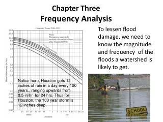
4. Frequency Analysis • Hydrologic systems are sometimes impacted by extreme events such as severe storms, floods, and droughts. • The magnitude of an extreme events occurring less frequently than more moderate events. • The objective of frequency analysis of hydrologic data is to relate the magnitude of extreme events to their frequency of occurrence through the use of probability distributions.

5. Frequency Analysis • The results of flood flow frequency analysis can be used for many engineering purposes; • 1) for the design of dams, bridges, culvert, and flood control structures. • 2) to determine the economic value of flood control projects. • 3) to delineate flood plains. • 4) to determine the effect of encroachments on the flood plain.

6. Return Period • Suppose that an extreme event is defined to have occurred if a random variable X is greater than or equal to some level xTr. The recurrence interval, is the time between occurrences of X  xTr

7. Return Period The record of annual maximum discharges of the Guadalupe River near Victoria, Texas

8. Return Period

9. Return Period If xTr = 50,000 cfs It can be seen that the maximum discharge exceeded this level 9 times during the period of record, with recurrence intervals ranging from 1-16 years. The return period Tr of the event X  xTr is the expected value of , E(). Its average value measured over a very large number of the occurrences. Therefore, the return period of a 50,000 cfs annual maximum discharge on the Guadalupe River is approximately  = 41/8 = 5.1 years

10. Return Period Thus , “the return period of an event of a given magnitude may be defined as the average recurrence interval between events equalling or exceeding a specified magnitude”. The probability of occurrence of the event X  xTr in any observation is Hence, E() = Tr = 1/p

11. Return Period The probability of occurrence of an event in any observation is the inverse of its return period. For example, the probability that the maximum discharge in the Guadalupe River will equal or exceed 50,000 cfs in any year is approximately

12. Return Period What is the probability that a Tr-year return period event will occur at least once in N years? P(X < xTr each year for N years) = (1-p)N P(X  xTr at least once in N years) = 1-(1-p)N or P(X  xTr at least once in N years) = 1-[1-(1/Tr)]N

13. Example 1 Estimate the probability that the annual maximum discharge Q on the Guadalupe River will exceed 50,000 cfs at least once during the next three years. Solution From the discussion above, P(Q  50,000 cfs in any year)  0.0195 So, P(Q  50,000 cfs at least once during the next 3 years) = 1-(1-0.195)3

14. Hydrologic Data Series Original Data Series • Complete Duration Series • consists of all the data. Original Data

15. Hydrologic Data Series Annual Exceedence Series • Partial Duration Series • is a series of data which are selected so their magnitude is greater than a predefined base value. If the base value is selected so that the number of values in the series is equal to the number of years of the record, the series is called anannual exceedence series.

16. Hydrologic Data Series Annual Maximum Series • Partial Duration Series • An extreme value series includes the largest and smallest values occurring in each of the equally-long time intervals of the record. The time interval length is usually taken as one year, and a series so selected is called annual series. • Using largest annual values, it is an annual maximum serie. • Selecting the smallest annual values produces an annual minimum series.

17. Hydrologic Data Series Original Data The annual maximum values and the annual exceedence values of the hypothetical data are arranged graphically in figure in order of magnitude. Magnitude Magnitude Annual Exceedence and maximum values

18. Extreme Value Distributions • The study of extreme hydrologic events involves the selection of a sequence of the largest or smallest observations from sets of data. • For example, Use just the largest flow recorded each year at a gaging station out of the many thousands of values recorded. Peak Flow Water level is usually recorded every 15 minutes, so there are 4x24 = 96 values recorded each day 365x96 = 35,040 values recorded each year Water Level

19. Extreme Value Distributions Extreme Value Type I PDF CDF : Extreme Value Type 1 Parameters :

20. Extreme Value Distributions Extreme Value Type I PDF Reduced Variate, y : CDF : Solving for y : Define y for Type II, Type II Distributions

21. Extreme Value Distributions More steeply Straight line Less steeply Variate, x Reduced Variate, y

22. Extreme Value Distributions Extreme Value Type I PDF Return Period : EV(I) Distribution, yTr : EV(I) Distribution, xTr :

23. Example 2 Annual maximum values of 10-minute duration rainfall at Chicago, illinois from 1913 to 1947 are presented in the table. Develop a model for storm rainfall frequency analysis using the Extreme Value Type I distribution and calculate the 5, 10, and 50 year return period maximum values of 10 minute rainfall at Chicago.

24. Example 2 Mean = 0.649 in Standard Deviation = 0.177 in

25. Example 2 Probability Model : To determine the values of xTr for Tr = 5 years :

26. Frequency Analysis using Frequency Factors The magnitude xtr of a hydrologic event can be represented as the mean plus the departure Dxtr of the variate from the mean. mean Departure KTr = Frequency Factor [Population] [Sample]

27. Frequency Analysis using Frequency Factors The theoretical K-Tr relationships for several probability distributions commonly used in hydrologic frequency analysis are now described.

28. Frequency Analysis using Frequency Factors Normal Distribution Frequency Factor : Value z : When p > 0.5, 1-p is substituted for p in equation * and the value of z computed by equation ** is given a negative sign.

29. Example 3 Calculate the frequency factor for the Normal Distribution for an event with a return period of 50 years. Solution For Tr = 50 years, p = 1/50 = 0.02

30. Frequency Analysis using Frequency Factors Extreme Value (I) Distribution Frequency Factor : Return Period :

31. Example 4 Determine the 5 year return period rainfall for Chicago using the frequency factor of Extreme Value (I) Distribution and the annual maximum rainfall data given in the table. Solution For Tr = 5 years

32. Frequency Analysis using Frequency Factors Log-Peason (III) Distribution Frequency Factor : where

33. Frequency Analysis Using Frequency Factors Positive Skew Negative Skew

34. Example 5 Calculate the 5 and 50 year return period annual maximum discharge of the Guadalupe River near Victoria, Texas, using the Log-Normal and Log-Pearson Type III Distributions. The data from 1935 to 1978 are given in the table. Solution The logarithms of the discharge values are taken and their statistics are calculated:

35. Extreme Value Distributions Log-Normal Distribution : Log-Pearson Type III Distribution :

36. Extreme Value Distributions