FREQUENCY ANALYSIS

1. FREQUENCY ANALYSIS • Basic Problem: To relate the magnitude of extreme events to their frequency of occurrence through the use of probability distributions.

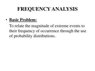
2. FREQUENCY ANALYSIS • Basic Assumptions: (a) Data analyzed are to be statistically independent & identically distributed - selection of data (Time dependence, time scale, mechanisms). (b) Change over time due to man-made (eg. urbanization) or natural processes do not alter the frequency relation - temporal trend in data (stationarity).

3. FREQUENCY ANALYSIS • Practical Problems: (a) Selection of reasonable & simple distribution. (b) Estimation of parameters in distribution. (c) Assessment of risk with reasonable accuracy.

4. REVIEW OF BASIC CONCEPTS Probabilistic Outcome of a hydrologic event (e.g., rainfall amount & duration; flood peak discharge; wave height, etc.) is random and cannot be predicted with certainty. Terminologies - Population The collection of all possible outcomes relevant to the process of interest. Example: (1) Max. 2-hr rainfall depth: all non-negative real numbers; (2) No. of storm in June: all non-negative integer numbers. - Sample A measured segment (or subset) of the population.

5. REVIEW OF BASIC CONCEPTS Terminologies - Random Variable A variable describable by a probability distribution which specifies the chance that the variable will assume a particular value. Convention: Capital letter for random variables (say, X) whereas the lower case letter (say, x) for numerical realization that the random variable X will take. Example: X = rainfall amount in 2 hours (a random variable) ; x = 100.2 mm/2hr (realization). - Random variables can be - discrete (eg., no. of rainy days in June) or - continuous (eg., max. 2-hr rainfall amount, flood discharge)..

6. REVIEW OF BASIC CONCEPTS Terminologies Frequency & Relative Frequency • For discrete random variables: • Frequency is the number of occurrences of a specific event. Relative frequency is resulting from dividing frequency by the total number of events. e.g. n = no. of years having exactly 50 rainy days; N = total no. of years. Let n=10 years and N=100 years. Then, the frequency of having exactly 50 rainy days is 10 and the relative frequency of having exactly 50 rainy days in 100 years is n/N = 0.1. • For continuous random variables: • Frequency needs to be defined for a class interval. • A plot of frequency or relative frequency versus class intervals is called histogram or probability polygon. • As the number of sample gets infinitely large and class interval length approaches to zero, the histogram will become a smooth curve, called probability density function.

7. REVIEW OF BASIC CONCEPTS Terminologies Probability Density Function (PDF) – • For a continuous random variable, the PDF must satisfy and f(x) ≥ 0 for all values of x. • For a discrete random variable, the PDF must satisfy and 1≥ p(x) ≥ 0for all values of x.

8. REVIEW OF BASIC CONCEPTS Terminologies - Cumulative Distribution Function - For a continuous random variable, For a discrete random variable, by

9. Statistical Properties of Random Variables • Population - Synonymous to sample space, which describes the complete assemblage of all the values representative of a particular random process. • Sample - Any subset of the population. • Parameters - Quantities that are descriptive of the population in a statistical model. Normally, Greek letters are used to denote statistical parameters. • Sample statistics (or simply statistics): Quantities calculated on the basis of sample observations.

10. Statistical Moments of Random Variables • Descriptors commonly used to show statistical properties of a RV are those indicative (1) Central tendency; (2) Dispersion; (3) Asymmetry. • Frequently used descriptors in these three categories are related to statistical moments of a RV. • Two types of statistical moments are commonly used in hydrosystem engineering applications: (1) product-moments and (2) L-moments.

11. Product-Moments • rth-order product-moment of X about any reference point X=xo is defined, for continuous case, as whereas for discrete case, where E[×] is a statistical expectation operator. • In practice, the first three moments (r=1, 2, 3) are used to describe the central tendency, variability, and asymmetry. • Two types of product-moments are commonly used: • Raw moments:µr'=E[Xr] rth-order moment about the origin; and • Central moments:µr=E[(Xµx)r] = rth-order central moment • Relations between two types of product-moments are: . where Cn,x = binomial coefficient = n!/(x!(n-x)!) • Main disadvantages of the product-moments are: (1) Estimation from sample observations is sensitive to the presence of outliers; and (2) Accuracy of sample product-moments deteriorates rapidly with increase in the order of the moments.

12. Mean, Mode, Median, and Quantiles • Expectation (1st-order moment) measures central tendency of random variable X • Mean (m) = Expectation = l1 = location of the centroid of PDF or PMF. • Two operational properties of the expectation are useful: in which mk=E[Xk] for k = 1,2, …, K. • For independent random variables, • Mode (xmo) - the value of a RV at which its PDF is peaked. The mode, xmo, can be obtained by solving • Median (xmd) - value that splits the distribution into two equal halves, i.e, • Quantiles - 100pth quantile of a RV X is a quantity xp that satisfies P(X £xp) = Fx(xp) = p • A PDF could be uni-modal, bimodal, or multi-modal. Generally, the mean, median, and mode of a random variable are different, unless the PDF is symmetric and uni-modal.

13. Uni-modal and bi-modal distributions

14. Variance, Standard Deviation, and Coefficient of Variation • Variance is the second-order central moment measuring the spreading of a RV over its range, • Standard deviation (sx) is the positive square root of the variance. • Coefficient of variation, Wx=sx/mx, is a dimensionless measure; useful for comparing the degree of uncertainty of two RVs with different units. • Three important properties of the variance are: • (1) Var[c] = 0 when c is a constant. • (2) Var[X] = E[X2] E2[X] • For multiple independent random variables, where ak=a constant and sk = standard deviation of Xk, k=1,2, ..., K.

15. Skewness Coefficient • Measures asymmetry of the PDF of a random variable • Skewness coefficient, gx, defined as • The sign of the skewness coefficient indicates the degree of symmetry of the probability distribution function. • Pearson skewness coefficient – • In practice, product-moments higher than 3rd-order are less used because they are unreliable and inaccurate when estimated from a small number of samples • See Table for equations to compute the sample product-moments.

16. Relative locations of mean, median, and mode for positively-skewed, symmetric, and negatively-skewed distributions.

17. Product-moments of random variables

18. Kurtosis(kx) • Measure of the peakedness of a distribution. • Related to the 4th central product-moment as • For a normal RV, its kurtosis is equal to 3. Sometimes, coefficient of excess, ex=kx3, is used. • All feasible distribution functions, skewness coefficient and kurtosis must satisfy

19. Some Commonly Used Distributions • NORMAL DISTRIBUTION Standardized Variable: Z has mean 0 and standard deviation 1.

20. Some Commonly Used Distributions • STANDARD NORMAL DISTRIBUTION:

21. x=1.3 x =4.50 x=0.3 x=0.6 x =2.25 x =1.65 (a) mx = 1.0 1.6 1.4 1.2 1.0 0.8 fLN(x) 0.6 0.4 0.2 0.0 0 1 2 3 4 5 6 x 0.7 0.6 0.5 0.4 fLN(x) 0.3 0.2 0.1 0 0 1 2 3 4 5 6 x Some Commonly Used Distributions • LOG-NORMAL DISTRIBUTION (b) Wx = 1.30

22. Some Commonly Used Distributions • Gumbel (Extreme-Value Type I) Distribution

23. 0.30 b=4, a=1 0.25 b=1, a=4 0.20 fG(x) 0.15 b=2, a=4 0.10 0.05 0.00 0 2 4 6 8 10 12 14 x Some Commonly Used Distributions • Log-Pearson Type 3 Distribution

24. Some Commonly Used Distributions • Log-Pearson Type 3 Distribution with a>0, x³ex when b>0 and with a>0, x£ex when b<0