Download
1 / 33
330 likes | 442 Vues
This paper presents advanced flow modelling techniques using SUTRA in heterogeneous porous media. It investigates the correlation of temperature gradients and wellbore porosity, with applications in geothermal energy extraction near the Waikato River and Taupo Volcanic Zone. The study emphasizes the importance of understanding in-situ fluid flow and permeability distributions for effective drilling strategies. Key findings include the relationship between porosity and permeability, and the implications for performance metrics in geothermal resource management.

E N D
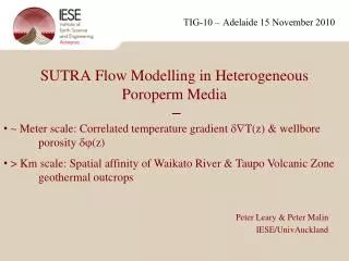
TIG-10 –Adelaide 15 November 2010 SUTRA Flow Modelling in Heterogeneous Poroperm Media– • ~ Meter scale: Correlated temperature gradient T(z) & wellbore porosity (z) • > Km scale: Spatial affinity of Waikato River & Taupo Volcanic Zone geothermal outcrops Peter Leary & Peter Malin IESE/UnivAuckland
Some geothermal/flow numbers: • 1 MWth ~ 4T(oC)/1000 V(ℓ/s) • 1 MWe ~ 4/100 V(ℓ/s) V(ℓ/s) ~ 25ℓ/s @ T=100oC • 10ℓ/s ~ 5400bbl/day • 50yr average US oil well production ~ 15±5bbl/day • 1ℓ oil ≡ 50¢ • 1ℓ hot water ≡ 0.5¢
Geothermal energy ≡ in situ fluid flow Flow rate/MWe ~ 25ℓ/s ~ 1000 times > oil formation flow rate Need to understand in situ flow.......
‘Laws’ of in situ fluid flow • Well-log ‘law’: power spectra scale inversely with spatial frequency: • S(k) ~ 1/k (=1/f-noise) • ~1/km < k < ~1/cm • Well-core ‘law’: porosity φ controls permeability κ: • δφ ~ δlog(κ)
Combine well-log & ‘well-core ‘laws’ in 3D realisation of in situ permeability distributions (where to aquifer access drill wells?)
Second realisation of well-log & ‘well-core ‘laws’ for in situ permeability distributions (where to drill wells?)
Fault realisation of well-log & ‘well-core ‘laws’ for in situ permeability distributions -- can geophysical methods tell where to drill?
SUTRA detailed flow modelling • M-scale spatial poroperm fluctuations: • Correlated temperature gradient T(z) & wellbore porosity (z), MWX field site, Colorado tight gas sands • KM-scale spatial poroperm fluctuations: • Spatial affinity of Waikato River for Taupo Volcanic Zone geothermal outcrops – evidence for joint fault control of geothermal circulation & river course?
MWX well spatial correlation of wellbore temperature gradient (red) with wellbore neutron porosity (blue) Temperature Gradient Porosity 1700m DEPTH IN WELL 2450m
Analytic solution: T(z)pred Pe(T(z)–T0)/h(z)obs T(z)obs (z)obs
Conductive + Advective heat flowQKT - C(T–T0) • Constant heat flow: δQ 0 δTC(T–T0)/Kδ • Darcy flow: /P g/δ (g/) δ • In situ permeability: 0exp() = 0exp() = • Pe= C2gh0/K ~ 1: • T(z) (T(z)–T0)/h(z)
SUTRA flow/transport solver computes temperature field fluctuations due to heat advected by water percolating through in situ (1/f-noise) poroperm medium.Find: • Thermal field fluctuates with porosity field • Wellbore fluctuations reflect 1/f-noise poroperm spatial fluctuations • Flow simulations with invalid synthetic fracture distributions give • inaccurate flow results
1/F-NOISE POROSITY DISTRIBUTION 20 40 60 80 100 120 0 20 40 60 80 100 120 140
0 0 0 0 0 0 0 0 0 0 0 0 20 20 20 20 20 20 20 20 20 20 20 20 40 40 40 40 40 40 40 40 40 40 40 40 60 60 60 60 60 60 60 60 60 60 60 60 80 80 80 80 80 80 80 80 80 80 80 80 100 100 100 100 100 100 100 100 100 100 100 100 120 120 120 120 120 120 120 120 120 120 120 120 -5 0 5 -5 0 5 -5 0 5 -5 0 5 -5 0 5 -5 0 5 -5 0 5 -5 0 5 -5 0 5 -5 0 5 -5 0 5 -5 0 5 Advective Heat Flow Conductive Heat Flow T(z) (red) --(z) (blue)
0 0 0 0 0 0 0 0 0 0 0 0 20 20 20 20 20 20 20 20 20 20 20 20 40 40 40 40 40 40 40 40 40 40 40 40 60 60 60 60 60 60 60 60 60 60 60 60 80 80 80 80 80 80 80 80 80 80 80 80 100 100 100 100 100 100 100 100 100 100 100 100 120 120 120 120 120 120 120 120 120 120 120 120 -5 0 5 -5 0 5 -5 0 5 -5 0 5 -5 0 5 -5 0 5 -5 0 5 -5 0 5 -5 0 5 -5 0 5 -5 0 5 -5 0 5 Advective Heat Flow in Poroperm Noise Gaussian Brownian T(z) (red) --(z) (blue)
T(z)obs T(z)pred Pe(T(z)–T0)/h(z)obs T(z)pred T(z)obs (z)obs
Synthetic Fracture Set Invalid Observed spatial correlation of in situ fractures requires porosity fluctuation power to scale inversely with spatial frequency (1/f-noise poroperm distribution): S(k) ~ 1/k, 1/km < k < 1/cm Synthetic fracture sets fail this spatial correlation criterion
Outcrop-based fracture-intercept basis for 3D synthetic fracture distribution
Sample Fourier power-spectra S(k) ~ kβ of borehole spatial fluctuations through synthetic fracture distribution with estimated exponents β
Distribution of Fourier power-spectra S(k) ~ kβ exponents β Synthetic data exponents: β ~ -0.4 +/- 0.3 Observed data exponents: β ~ -1.1 +/- 0.15
SUTRA detailed flow modelling • M-scale spatial poroperm fluctuations: • Correlated temperature gradient T(z) & wellbore porosity (z), MWX field site, Colorado tight gas sands • KM-scale spatial poroperm fluctuations: • Spatial affinity of Waikato River for Taupo Volcanic Zone geothermal outcrops – evidence for joint fault control of geothermal circulation & river course?
XFlt No XFlt
M-scale Summary/Conclusions • Sutra fluid flow/transport simulator reproduces spatial correlation between fluctuations in thermal gradient and porosity observed in MWX well advective/percolation heat transport • Thermal gradient fluctuations track in situ porosity fluctuations • Observed thermal gradient fluctuations ~ 1/f-noise spatial correlation • Observed advection shows bulk permeability fluctuations ~ 1/f-noise • Standard fracture simulation S\W fail to meet the observed 1/f-noise spatial correlation criterion • Flow simulators operating with incorrect fracture spatial correlations cannot give accurate flow/transport results
> KM-scale Summary/Conclusions • Sutra fluid flow/transport simulator indicates increased fault-borne • heat transport where faults cross • Thermal diffusion from crossed-fault ‘thermal plumes’ may account for the circular geometry and location of TVZ geothermal outcrops • Faults that (may) control the location of TVZ geothermal outcrops may also guide the course of the Waikato River in the central TVZ • Detailed physically-based flow modelling of fracture/fault borne heat advection in the central TVZ may help understanding of geothermal fields in general • If faults are key structures in TVZ geothermal outcrops, faults are also likely to be key structures in, say, Australian HSA plays; locating in situ buried faults could be important to HSA economics.