Discrete Probability Distributions

1. Chapter 5 Discrete Probability Distributions

2. Objectives In this chapter, you learn: • The properties of a probability distribution. • To compute the expected value and variance of a probability distribution. • To compute probabilities from binomial, and Poisson distributions. • To use the binomial, and Poisson distributions to solve business problems

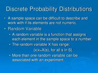
3. Definitions • Discrete variables produce outcomes that come from a counting process (e.g. number of classes you are taking). • Continuous variables produce outcomes that come from a measurement (e.g. your annual salary, or your weight).

4. Types Of Variables Types Of Variables Discrete Variable Continuous Variable Ch. 5 Ch. 5 Ch. 5 Ch. 6 Ch. 6 Ch. 6

5. Discrete Variables • Can only assume a countable number of values Examples: • Roll a die twice Let X be the number of times 4 occurs (then X could be 0, 1, or 2 times) • Toss a coin 5 times. Let X be the number of heads (then X = 0, 1, 2, 3, 4, or 5)

6. A probability distribution for a discrete variable is a mutually exclusive listing of all possible numerical outcomes for that variable and a probability of occurrence associated with each outcome. Probability Distribution For A Discrete Variable

7. Probability Distributions Are Often Represented Graphically

8. Discrete Variables Expected Value (Measuring Center) • Expected Value (or mean) of a discrete variable (Weighted Average)

9. Discrete Variables: Measuring Dispersion • Variance of a discrete variable • Standard Deviation of a discrete variable where: E(X) = Expected value of the discrete variable X xi = the ith outcome of X P(X=xi) = Probability of the ith occurrence of X

10. Discrete Variables: Measuring Dispersion (continued)

11. Probability Distributions Ch. 5 Discrete Probability Distributions Continuous Probability Distributions Ch. 6 Binomial Normal Poisson Probability Distributions

12. Binomial Probability Distribution • A fixed number of observations, n • e.g., 15 tosses of a coin; ten light bulbs taken from a warehouse • Each observation is categorized as to whether or not the “event of interest” occurred • e.g., head or tail in each toss of a coin; defective or not defective light bulb • Since these two categories are mutually exclusive and collectively exhaustive • When the probability of the event of interest is represented as π, then the probability of the event of interest not occurring is 1 - π • Constant probability for the event of interest occurring (π) for each observation • Probability of getting a tail is the same each time we toss the coin

13. Binomial Probability Distribution (continued) • Observations are independent • The outcome of one observation does not affect the outcome of the other • Two sampling methods deliver independence • Infinite population without replacement • Finite population with replacement

14. Possible Applications for the Binomial Distribution • A manufacturing plant labels items as either defective or acceptable • A firm bidding for contracts will either get a contract or not • A marketing research firm receives survey responses of “yes I will buy” or “no I will not” • New job applicants either accept the offer or reject it

15. The Binomial DistributionCounting Techniques • Suppose the event of interest is obtaining heads on the toss of a fair coin. You are to toss the coin three times. In how many ways can you get two heads? • Possible ways: HHT, HTH, THH, so there are three ways you can getting two heads. • This situation is fairly simple. We need to be able to count the number of ways for more complicated situations.

16. Counting TechniquesRule of Combinations • The number of combinations of selecting x objects out of n objects is where: n! =(n)(n - 1)(n - 2) . . . (2)(1) x! = (X)(X - 1)(X - 2) . . . (2)(1) 0! = 1 (by definition)

17. How many possible 3 scoop combinations could you create at an ice cream parlor if you have 31 flavors to select from and no flavor can be used more than once in the 3 scoops? The total choices is n = 31, and we select X = 3. Counting TechniquesRule of Combinations

18. Binomial Distribution Formula n ! - x x n P(X=x |n,π) = π (1-π) x! ( - ) n x ! P(X=x|n,π) = probability of x events of interest in ntrials, with the probability of an “event of interest” being πfor each trial x = number of “events of interest” in sample, (x = 0, 1, 2, ...,n) n = sample size (number of trials or observations) π = probability of “event of interest” Example: Flip a coin four times, let x = # heads: n= 4 π= 0.5 1 - π= (1 - 0.5) = 0.5 X = 0, 1, 2, 3, 4

19. Example: Calculating a Binomial Probability What is the probability of one success in five observations if the probability of an event of interest is 0.1? x = 1, n = 5, and π = 0.1

20. The Binomial DistributionExample Suppose the probability of purchasing a defective computer is 0.02. What is the probability of purchasing 2 defective computers in a group of 10? x = 2, n = 10, and π = 0.02

21. The Binomial Distribution Shape • The shape of the binomial distribution depends on the values of π and n • Here, n = 5 and π = .1 • Here, n = 5 and π = .5

22. The Binomial Distribution Using Binomial Tables (Available On Line) Examples: n = 10, π = 0.35, x = 3: P(X = 3|10, 0.35) = 0.2522 n = 10, π = 0.75, x = 8: P(X = 8|10, 0.75) = 0.2816

23. Binomial Distribution Characteristics • Mean • Variance and Standard Deviation Where n = sample size π = probability of the event of interest for any trial (1 – π) = probability of no event of interest for any trial

24. The Binomial DistributionCharacteristics Examples

25. The Poisson DistributionDefinitions • You use the Poisson distribution when you are interested in the number of times an event occurs in a given area of opportunity. • An area of opportunity is a continuous unit or interval of time, volume, or such area in which more than one occurrence of an event can occur. • The number of scratches in a car’s paint • The number of mosquito bites on a person • The number of computer crashes in a day

26. The Poisson Distribution • Apply the Poisson Distribution when: • You wish to count the number of times an event occurs in a given area of opportunity • The probability that an event occurs in one area of opportunity is the same for all areas of opportunity • The number of events that occur in one area of opportunity is independent of the number of events that occur in the other areas of opportunity • The probability that two or more events occur in an area of opportunity approaches zero as the area of opportunity becomes smaller • The average number of events per unit is (lambda)

27. Poisson Distribution Formula where: x = number of events in an area of opportunity  = expected number of events e = base of the natural logarithm system (2.71828...)

28. Poisson Distribution Characteristics • Mean • Variance and Standard Deviation where  = expected number of events

29. Using Poisson Tables (Available On Line) Example: Find P(X = 2 |  = 0.50)

30. Graph of Poisson Probabilities Graphically:  = 0.50 P(X = 2 | =0.50) = 0.0758

31. Poisson Distribution Shape • The shape of the Poisson Distribution depends on the parameter  :  = 3.00  = 0.50

32. Chapter Summary In this chapter we covered: • The properties of a probability distribution. • To compute the expected value and variance of a probability distribution. • To compute probabilities from binomial, and Poisson distributions. • To use the binomial, and Poisson distributions to solve business problems