Discrete Probability Distributions

1. Discrete Probability Distributions Unit 4

2. Introduction • Many decisions in business, insurance, and other real-life situations are made by assigning probabilities to all possible outcomes pertaining to the situation and then evaluating the results. For example, a saleswomen can compute the probability that she will make 0,1,2 or 3 or more sales in a single day. An insurance company might be able to assign probabilities to the number of vehicles a family owns. Once these probabilities are assigned, statistics such as mean, variance and standard deviations can be computed for these events. With these statistics, various decisions can be made.

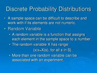
3. Vocabulary • Random Variable – is a variable whose value are determined by chance. • There are two types of random variables • Discrete – a random variable that has a finite or an infinite number of values that can be counted. (A die is rolled and X can represent the number outcomes 1,2,3,4,5 & 6) • Continuous – variables that can assume all values in the interval between any two given values. Continuous random variables are obtained from data that can be measured rather than counted. (heights, weights, temperature and time)

4. Probability Distributions for Discrete Random Variables • Tossing three coins • Sample Space: TTT, TTH, THT, HTT, HHT, HTH, THH, HHH. • X is the random variable for the number of heads, then X assumes the values of 0,1,2,& 3. • Probability for the values of X can be determined as follows: • 0 heads = 1/8, 1 head =3/8 2 heads = 3/8 and 3 heads = 1/8 • From these values, a probability distribution can be constructed by listing the outcomes and assigning the probability of each outcome.

5. Probability Distribution for a Discrete Probability Distribution

6. Definition • A Discrete Probability Distribution - consists of the values a random variable can assume and the corresponding probabilities of the values. The probabilities are determined theoretically or by observation. • Can be shown by a table or a graph

7. Construct a Probability Distribution for rolling a single die Probability Distributions can be shown graphically by representing the values of X on the x axis and the probabilities P(X) on the y axis .

8. Theoretical Probability Distributions • The two examples we just looked are examples of theoretical probability distributions. We did not need to perform the experiments to compute the probabilities. In contrast to construct actual probability distributions, you must observe the variable over a period of time. That would then be empirical.

9. Baseball World Series • Then baseball World Series is played by the winner of the National League and the American League. The first team to win four games wins the World Series. The series consists of 4-7 games depending on the individual victories.

10. The data shown consists of the number of games played in the World Series from 1965 to 2005 *no game 1994

11. Construct a Probability Distribution of the World Series data

12. Graph the Probability Distribution

13. Probability Distribution Requirements • Two Requirements • The sum of the probabilities of all the events in the sample space must equal 1; that is ΣP(X)=1 • The probability of each event in the sample space must be between or equal to 0 and 1. That is , 0≤ P(X)≤1 • A probability cannot be a number greater than 1 or a negative number

14. Determine whether each distribution is a probability distribution

15. Mean, Variance, Standard Deviation, and Expectation 4-2

16. Introduction • The mean, variance, and standard deviation for a probability distribution are computed differently from the mean, variance, and standard deviation for samples. This section explains how these measures – as well as a new measure called expectation – are calculated for probability distributions.

17. Mean for Probability Distributions • Previously the mean for a sample or population was computed by adding the values and dividing by the total number of values. • But how would you compute the mean of the number of spots that show on top when a die is rolled? You could try rolling the die, say, 10 times, recording the number of spots, and finding the mean; however, this answer would only approximate the true mean. What about 50 rolls or 100 rolls? Actually, the more times the die is rolled , the better the approximation.

18. Mean for Probability Distributions • You might ask, then, How many times must the die be rolled to get the exact answer? It must be rolled an infinite number of times. Since this task is impossible, the previous formulas cannot be used because the denominators would be infinity. Hence, we need a new method of computing the mean. This method gives the exact theoretical value of the mean as if it were possible to roll the die an infinite number of times.

19. Example • Suppose two coins are tossed repeatedly, and the number of heads that occurred is recorded. What will be the mean of the number of heads? The sample space is HH, HT, TH, TT and each outcome has a probability of ¼ . Now, in the long run, you would expect two heads (HH) to occur approximately ¼ of the time, one head to occur approximately ½ of the time (HT or TH), and no heads (TT) to occur approximately ¼ of the time. So the formula would look like this¼ * 2 + ½ * 1 + ¼ * 0 = 1 • That is, if it were possible to toss the coins many times or an infinite number of times, the average of the number of heads would be 1.

20. Formula • To find the mean for a probability distribution, you must multiply each possible outcome by its corresponding probability and find the sum of the products.

21. Rounding Rule for the Mean, Variance and Standard Deviation for a Probability Distribution • The rounding rule for the mean, variance, and standard deviation for variables of a probability distribution is this: The mean, variance, and standard deviation should be rounded to one more decimal place than the outcome X. When fractions are used, they should be reduced to lowest terms. Let’s go Practice….

22. Example 1 – Find the mean of the number of spots that appear when a die is rolled. P(X) = 1 * 1/6 + 2 * 1/6 + 3 * 1/6 + 4 * 1/6 + 5 * 1/6 + 6 * 1/6 = 21/6 = 3 ½ 0R 3.5 This means that that when a die is tossed many times, the theoretical mean will be 3.5, even though a die can not roll a 3.5, the theoretical average is 3.5.

23. Example 2 – In a family with two children, find the mean of the number of children who will be girls. P(X) = 0 * ¼ + 1 * ½ + 2 * ¼ = 1

24. Example 3- If three coins are tossed, find the mean of the number of heads that occur.

25. Example 4 - Number of Trips of Five Nights or More The probability distribution shown represents the number of trips of five nights or more that American adults take per year. (That is, 6% do not take any trips lasting five nights or more, 70% take one trip lasting five nights or more per year, etc.) Find the mean.

26. Variance and Standard Deviation • For a probability distribution, the mean of the random variable describes the measure of the so-called long-run or theoretical average, but it does not tell anything about the spread of the distribution. Recall from our previous units that in order to measure this spread or variability, statisticians use the variance and standard deviation.

27. Variance and Standard Deviation • Our previous formulas cannot be used for a random variable of a probability distribution since N is infinite, so the variance and standard deviation must be computed differently. • To find the variance for the random variable of a probability distribution, subtract the theoretical mean of the random variable from each outcome and square the difference. Then multiply each difference by its corresponding probability and add the products.

28. Formula Remember that the variance and standard deviation cannot be negative.

29. Example 1 – Find the variance and standard deviation of the number of spots that appear when a die is rolled. Recall that the mean was 3.5 in this previous example. Square each outcome and multiply by the corresponding probability, sum those products, and then subtract the square of the mean. Variance = (12 * 1/6 + 22 * 1/6 + 32 * 1/6 + 42 * 1/6 + 52 * 1/6 + 62 * 1/6) – (3.5)2 = 2.9 Standard Deviation = √2.9 = 1.7

30. Example 2 –Selecting Numbered Balls. A box contains 5 balls. Two are numbered 3, one is numbered 4, and two are numbered 5. The balls are mixed and one is selected at random. After a ball is selected, its number is recorded. Then it is replaced. If the experiment is repeated many times, find the variance and standard deviation of the numbers on the balls. Calculate the mean: Calculate the variance: Calculate the standard deviation:

31. Example 3 – On Hold for Talk Radio A talk radio station has four telephone lines. If the host is unable to talk (i .e., during a commercial) or is talking to a person, the other callers are placed on hold. When all lines are in use, others who are trying to call in get a busy signal. The probability that 0, 1,2,3, or 4 people will get through is shown in the distribution. Find the mean, variance and standard deviation for the distribution. Should the radio station have considered getting more phone lines installed? Mean: Variance: Standard Deviation:

32. Expectation • Another concept related to the mean for a probability distribution is that of expected value or expectation. Expected value is used in various types of games of chance, in insurance, and in other areas, such as decision theory. • The formula for the expected value is the same as the formula for the theoretical mean. The expected value, then, is the theoretical mean of the probability distribution. • When expected value problems involve money, it is customary to round the answer to the nearest cent.

33. Example 1 – Winning Tickets One thousand tickets are sold at $1 each for a color television valued at $350. What is the expected value of the gain if you purchase one ticket? Two things should be noted. First, for a win, the net gain is $349, since you do not get the cost of the ticket ($1) back. Second, for a loss, the gain is represented by a negative number, in this case - $ 1.

34. Expectations • Note that the expectation is - $0.65. This does not mean that you lose $0.65, since you can only win a television set valued at $350 or lose $1 on the ticket. What this expectation means is that the average of the losses is $0.65 for each of the 1000 ticket holders. • Here is another way of looking at this situation: If you purchased one ticket each week over a long time, the average loss would be $0.65 per ticket, since theoretically, on average, you would win the set once for each 1000 tickets purchased.

35. Example 2 – Winning Tickets One thousand tickets are sold at $1 each for four prizes of $100, $50, $25, and $10. After each prize drawing, the winning ticket is then returned to the pool of tickets. What is the expected value if you purchase two tickets?

36. Example 3 – Bond Investment A financial adviser suggests that his client select one of two types of bonds in which to invest $5000. Bond X pays a return of 4% and has a default rate of 2%. Bond Y has a 2 ½ % return and a default rate of 1 %. Find the expected rate of return and decide which bond would be a better investment. When the bond defaults, the investor loses all the investment. The return on bond X is $5000 * 4% = $200. The expected return then is E(X) = $200(0.98) - $5000(0.02) = $96 The return on bond Y is $5000 * 2 ½ % = $125. The expected return then is E(X) =$125(0.99) - $5000(0.01) = $73.75 Hence, bond X would be a better investment since the expected return is higher.