Download
1 / 24
240 likes | 437 Vues
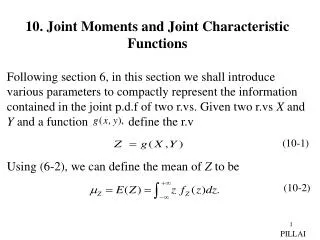
10. Joint Moments and Joint Characteristic Functions. Following section 6, in this section we shall introduce various parameters to compactly represent the information contained in the joint p.d.f of two r.vs. Given two r.vs X and Y and a function define the r.v

E N D
10. Joint Moments and Joint Characteristic Functions Following section 6, in this section we shall introduce various parameters to compactly represent the information contained in the joint p.d.f of two r.vs. Given two r.vs X and Y and a function define the r.v Using (6-2), we can define the mean of Z to be (10-1) (10-2) PILLAI
However, the situation here is similar to that in (6-13), and it is possible to express the mean of in terms of without computing To see this, recall from (5-26) and (7-10) that where is the region in xy plane satisfying the above inequality. From (10-3), we get As covers the entire z axis, the corresponding regions are nonoverlapping, and they cover the entire xy plane. (10-3) (10-4) PILLAI
By integrating (10-4), we obtain the useful formula or If X and Y are discrete-type r.vs, then Since expectation is a linear operator, we also get (10-5) (10-6) (10-7) (10-8) PILLAI
If X and Y are independent r.vs, it is easy to see that and are always independent of each other. In that case using (10-7), we get the interesting result However (10-9) is in general not true (if X and Y are not independent). In the case of one random variable (see (10- 6)), we defined the parameters mean and variance to represent its average behavior. How does one parametrically represent similar cross-behavior between two random variables? Towards this, we can generalize the variance definition given in (6-16) as shown below: (10-9) PILLAI
Covariance: Given any two r.vs X and Y, define By expanding and simplifying the right side of (10-10), we also get It is easy to see that To see (10-12), let so that (10-10) (10-11) (10-12) (10-13) PILLAI
The right side of (10-13) represents a quadratic in the variable a that has no distinct real roots (Fig. 10.1). Thus the roots are imaginary (or double) and hence the discriminant must be non-positive, and that gives (10-12). Using (10-12), we may define the normalized parameter or and it represents the correlation coefficient between X and Y. (10-14) (10-15) Fig. 10.1 PILLAI
Uncorrelated r.vs: If then X and Y are said to be uncorrelated r.vs. From (11), if X and Y are uncorrelated, then Orthogonality: X and Y are said to be orthogonal if From (10-16) - (10-17), if either X or Y has zero mean, then orthogonality implies uncorrelatedness also and vice-versa. Suppose X and Y are independent r.vs. Then from (10-9) with we get and together with (10-16), we conclude that the random variables are uncorrelated, thus justifying the original definition in (10-10). Thus independence implies uncorrelatedness. (10-16) (10-17) PILLAI
Naturally, if two random variables are statistically independent, then there cannot be any correlation between them However, the converse is in general not true. As the next example shows, random variables can be uncorrelated without being independent. Example 10.1: Let Suppose X and Y are independent. Define Z = X + Y, W = X - Y . Show that Z and W are dependent, but uncorrelated r.vs. Solution: gives the only solution set to be Moreover and PILLAI
Fig. 10.2 Thus (see the shaded region in Fig. 10.2) and hence or by direct computation ( Z = X + Y ) (10-18) PILLAI
(10-19) and Clearly Thus Z and W are not independent. However and and hence implying that Z and W are uncorrelated random variables. (10-20) (10-21) (10-22) PILLAI
Example 10.2: Let Determine the variance of Z in terms of and Solution: and using (10-15) In particular if X and Y are independent, then and (10-23) reduces to Thus the variance of the sum of independent r.vs is the sum of their variances (10-23) (10-24) PILLAI
Moments: represents the joint moment of order (k,m) for X and Y. Following the one random variable case, we can define the joint characteristic function between two random variables which will turn out to be useful for moment calculations. Joint characteristic functions: The joint characteristic function between X and Y is defined as Note that (10-25) (10-26) PILLAI
It is easy to show that If X and Y are independent r.vs, then from (10-26), we obtain Also More on Gaussian r.vs : From Lecture 7, X and Y are said to be jointly Gaussian as if their joint p.d.f has the form in (7-23). In that case, by direct substitution and simplification, we obtain the joint characteristic function of two jointly Gaussian r.vs to be (10-27) (10-28) (10-29) PILLAI
(10-30) Equation (10-14) can be used to make various conclusions. Letting in (10-30), we get and it agrees with (6-47). From (7-23) by direct computation using (10-11), it is easy to show that for two jointly Gaussian random variables Hence from (10-14), in represents the actual correlation coefficient of the two jointly Gaussian r.vs in (7-23). Notice that implies (10-31) PILLAI
Thus if X and Y are jointly Gaussian, uncorrelatedness does imply independence between the two random variables. Gaussian case is the only exception where the two concepts imply each other. Example 10.3: Let X and Y be jointly Gaussian r.vs with parameters Define Determine Solution: In this case we can make use of characteristic function to solve this problem. (10-32) PILLAI
From (10-30) with u and v replaced by au and bu respectively we get where Notice that (10-33) has the same form as (10-31), and hence we conclude that is also Gaussian with mean and variance as in (10-34) - (10-35), which also agrees with (10-23). From the previous example, we conclude that any linear combination of jointly Gaussian r.vs generate a Gaussian r.v. (10-33) (10-34) (10-35) PILLAI
In other words, linearity preserves Gaussianity. We can use the characteristic function relation to conclude an even more general result. Example 10.4: Suppose X and Y are jointly Gaussian r.vs as in the previous example. Define two linear combinations what can we say about their joint distribution? Solution: The characteristic function of Z and W is given by As before substituting (10-30) into (10-37) with u and v replaced by au + cv and bu + dv respectively, we get (10-36) (10-37) PILLAI
(10-38) where and From (10-38), we conclude that Z and W are also jointly distributed Gaussian r.vs with means, variances and correlation coefficient as in (10-39) - (10-43). (10-39) (10-40) (10-41) (10-42) (10-43) PILLAI
Linear operator Gaussian input Gaussian output To summarize, any two linear combinations of jointly Gaussian random variables (independent or dependent) are also jointly Gaussian r.vs. Of course, we could have reached the same conclusion by deriving the joint p.d.f using the technique developed in section 9 (refer (7-29)). Gaussian random variables are also interesting because of the following result: Central Limit Theorem: Suppose are a set of zero mean independent, identically distributed (i.i.d) random Fig. 10.3 PILLAI
variables with some common distribution. Consider their scaled sum Then asymptotically (as ) Proof: Although the theorem is true under even more general conditions, we shall prove it here under the independence assumption. Let represent their common variance. Since we have (10-44) (10-45) (10-46) (10-47) PILLAI
Consider where we have made use of the independence of the r.vs But where we have made use of (10-46) - (10-47). Substituting (10-49) into (10-48), we obtain and as (10-48) (10-49) (10-50) (10-51) PILLAI
since (10-52) [Note that terms in (10-50) decay faster than But (10-51) represents the characteristic function of a zero mean normal r.v with variance and (10-45) follows. The central limit theorem states that a large sum of independent random variables each with finite variance tends to behave like a normal random variable. Thus the individual p.d.fs become unimportant to analyze the collective sum behavior. If we model the noise phenomenon as the sum of a large number of independent random variables (eg: electron motion in resistor components), then this theorem allows us to conclude that noise behaves like a Gaussian r.v. PILLAI
It may be remarked that the finite variance assumption is necessary for the theorem to hold good. To prove its importance, consider the r.vs to be Cauchy distributed, and let where each Then since substituting this into (10-48), we get which shows that Y is still Cauchy with parameter In other words, central limit theorem doesn’t hold good for a set of Cauchy r.vs as their variances are undefined. (10-53) (10-54) (10-55) PILLAI
Joint characteristic functions are useful in determining the p.d.f of linear combinations of r.vs. For example, with X and Y as independent Poisson r.vs with parameters and respectively, let Then But from (6-33) so that i.e., sum of independent Poisson r.vs is also a Poisson random variable. (10-56) (10-57) (10-58) (10-59) PILLAI