
Hash Tables
E N D
Presentation Transcript
Ellen Walker CPSC 201 Data Structures Hiram College Hash Tables
Breaking the Rules • The fastest possible search algorithm, if you only compare two items at once, is O(log n) where n is the number of items in the table. • But, if we can figure out a way to compare multiple items at once, we can beat that!
Magic Address Calculator • Represent your table as an array • Add a new function, the “magic address calculator” • The input to this function is the key • The output of this function is the address to look in • No comparisons, so we’re not limited to log n. • In fact, if the calculator takes the same time for every input, it’s constant time search!
Hash Function • The “magic calculator” function is called a hash function • It treats the key as a sequence of bits or an integer, regardless of its original type • Example hash functions (not very good ones) • Last two digits of the integer (table size 100) • Divide the bit string into sequences of 8 bits and XOR all sequences together (table size 256)
Hash Table • Table is an array of TableSize, hash(key) is a function that returns a value from 0 to TableSize. • To insert: • Table[hash(key)] = key • To retrieve: • Result = Table[hash(key)] • To delete: • Table[hash(key)] = empty marker • Can it really be that simple?
Hash Table Collisions • If the size of the the table is smaller than the number of possible keys, then there must be at least two keys with the same hash value. • E.g. 202 and 102 if key is last 2 digits • If we want to insert both values, we will get a collision • The item we retrieve might not really have a matching key • The location to insert into might already be full
Avoiding Collisions • Make the table “big” (if you can afford it) • Pick the right hash function • If you know all possible keys, create a perfect hash function (unique value for each possible key) • Try to distribute all possible keys evenly among the addresses • Try to distribute the most likely keys evenly among the addresses
Choosing a Hash Function • Should return integers in a fixed range • Should be quick to compute • Should avoid obvious patterns of results • Should involve the entire search key
Typical Hash Functions • Taking an integer modulo a prime number • Prime number has only 1 and itself as factors • This avoids patterns of addresses • Easiest to analyze and most common • Folding (integer or bits) • Divide value into subgroups (k bits or digits) • Add or XOR together subgroups
Resolving Collisions byOpen Addressing • Find another place within the table for the item • Linear probing: new item goes in first empty space after the result of the hash function (Offsets are sequence of numbers) • Quadratic probing: first look in next space, then skip to 4th space, then 9th, then 16th, etc. (Offsets are sequence of squares) • Double hashing: use a second hash function on the key to find the offset. (Offsets are multiples of the second hash value)
Insertion with Open Addressing void insert(E item){ int address = hash(item); while(Table[address]!=null){ compute next offset address = address + offset } Table[address] = item; }
Retrieval with Open Addressing E retrieve(E item){ int address = hash(item); while((!table[address].equals(item))&& (table[address] != null)){ compute next offset address = address + offset } return( table[address]); //returns null if not found }
Issues with Open Addressing • Retrieval must follow same sequence of probes as insertion • If a collision fills a cell, then it forces a collision with the value that hashes directly to the cell. • Consider: • Hash(key) = key%11 • Sequence of items: 1,14,12,2,3,41,27,15 • Try linear, quadratic, double hash = key%7
Comparing Open Addressing Schemes • Linear probing is most prone to clustering • Large clumps of cells fill, causing long sequences of probes for each insertion • Quadratic probing is less prone to clustering • Each probe is even further from the “cluster” • No guarantee every slot will be searched, though! • Double hashing depends on the other hash function • Its base should be relatively prime to the original base so there is no pattern • In this case, it is as good or better than quadratic
Restructuring the Hash Table • Each “address” can contain multiple items • Bucket (set max # items per hash key) • Separate chaining (array of linked lists) • Our example again: • Hash(key) = key%11 • Sequence of items: 1,14,12,2,3,41,27,15
Separate chaining • Hash table as array of linked lists
Growing a Hash Table • Open addressing: • When the hash table is full, allocate a bigger one. • “Rehashing” = add each element from the original table to the full one using the new hash code. • Chaining: • When the lists are getting too long, allocate a bigger table • Rehash as above.