GIS in Water Resources Midterm Review 2008

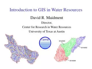
1. GIS in Water ResourcesMidterm Review 2008 David Maidment, David Tarboton and Ayse Irmak

2. Data Model Conceptual Model – a set of concepts that describe a subject and allow reasoning about it Mathematical Model – a conceptual model expressed in symbols and equations Data Model – a conceptual model expressed in a data structure (e.g. ascii files, Excel tables, …..) Geographic Data Model – a conceptual model for describing and reasoning about the world expressed in a GIS database

3. A geographicdata model is a structure for organizing geospatial data so that it can be easily stored and retrieved. Geographic coordinates Tabular attributes

4. Raster and Vector Data Raster data are described by a cell grid, one value per cell Vector Raster Point Line Zone of cells Polygon

5. Themes or Data Layers Vector data: point, line or polygon features How each of these features could be represented using vector or raster?

6. Workspace Geodatabase Feature Dataset Feature Class Geometric Network Relationship Object Class ArcGIS Geodatabase (what is in a geodatabase)

7. Geodatabase and Feature Dataset • A geodatabase is a relational database that stores geographic information. • A feature dataset is a collection of feature classes that share the same spatial reference frame.

8. Feature Class • A feature class is a collection of geographic objects in tabular format that have the same behavior and the same attributes. Feature Class = Object class + spatial coordinates

9. Object Class • An object class is a collection of objects in tabular format that have the same behavior and the same attributes (do not have a shape). An object class is a table that has a unique identifier (ObjectID) for each record

10. Relationship Relationship between spatial and non-spatial objects Water quality data (non-spatial) Measurement station (spatial)

11. Geodesy, Map Projections and Coordinate Systems • Geodesy - the shape of the earth and definition of earth datums • Map Projection - the transformation of a curved earth to a flat map • Coordinate systems - (x,y) coordinate systems for map data Spatial Reference = Datum + Projection + Coordinate system

12. Types of Coordinate Systems • (1) Global Cartesian coordinates (x,y,z) for the whole earth • (2) Geographic coordinates (f, l, z) • (3) Projected coordinates (x, y, z) on a local area of the earth’s surface • The z-coordinate in (1) and (3) is defined geometrically; in (2) the z-coordinate is defined gravitationally

13. Z Greenwich Meridian O • Y X Equator Global Cartesian Coordinates (x,y,z)

14. Geographic Coordinates (f, l, z) • Latitude (f) and Longitude (l) defined using an ellipsoid, an ellipse rotated about an axis • Elevation (z) defined using geoid, a surface of constant gravitational potential • Earth datums define standard values of the ellipsoid and geoid

15. Latitude and Longitude Longitude line (Meridian) N W E S Range: 180ºW - 0º - 180ºE Latitude line (Parallel) N W E S (0ºN, 0ºE) Equator, Prime Meridian Range: 90ºS - 0º - 90ºN

16. Latitude and Longitude in North America Austin: (30°N, 98°W) Logan: (42°N, 112°W) Lincoln: (40°N, 96° W 60 N 30 N 60 W 120 W 90 W 0 N

17. Length on Meridians and Parallels (Lat, Long) = (f, l) Length on a Meridian: AB = ReDf (same for all latitudes) R Dl D R 30 N C B Re Df 0 N Re Length on a Parallel: CD = R Dl = ReDl Cos f (varies with latitude) A

18. Example 1: What is the length of a 1º increment along on a meridian • and on a parallel at 30N, 90W? • Radius of the earth = 6370 km. • Solution: • A 1º angle has first to be converted to radians • p radians = 180 º, so 1º = p/180 = 3.1416/180 = 0.0175 radians • For the meridian, DL = ReDf = 6370 * 0.0175 = 111 km • For the parallel, DL = ReDl Cos f • = 6370 * 0.0175 * Cos 30 • = 96.5 km • Parallels converge as poles are approached

19. Example 2: What is the size of a 1 arc-second DEM cell when projected to (x,y) coordinates at 30º N? • Radius of the earth = 6370 km = 6,370,000m = 6.37 x 106 m • Solution: • A 1” angle has first to be converted to radians • p radians = 180 º, so 1” = 1/3600 º = (1/3600)p/180 radians = 4.848 x 10-6 radians • For the left and right sides, DL = ReDf = 6.37 x 106 * 4.848 x 10-6 =30.88m • For the top and bottom sides, DL = ReDl Cos f = 6.37 x 106 * 4.848 x 10-6 * Cos 30º = 30.88 x 0.8660 = 26.75m • Left and right sides of cell converge as poles are approached

20. Z B A  • Y X Curved Earth Distance(from A to B) Shortest distance is along a “Great Circle” A “Great Circle” is the intersection of a sphere with a plane going through its center. 1. Spherical coordinates converted to Cartesian coordinates. 2. Vector dot product used to calculate angle  from latitude and longitude 3. Great circle distance is R, where R=6370 km2 Longley et al. (2001)

21. Horizontal Earth Datums • An earth datum is defined by an ellipse and an axis of rotation • NAD27 (North American Datum of 1927) uses the Clarke (1866) ellipsoid on a non geocentric axis of rotation • NAD83 (NAD,1983) uses the GRS80 ellipsoid on a geocentric axis of rotation • WGS84 (World Geodetic System of 1984) uses GRS80, almost the same as NAD83

22. Vertical Earth Datums • A vertical datum defines elevation, z • NGVD29 (National Geodetic Vertical Datum of 1929) • NAVD88 (North American Vertical Datum of 1988) • takes into account a map of gravity anomalies between the ellipsoid and the geoid

23. Types of Projections • Conic (Albers Equal Area, Lambert Conformal Conic) - good for East-West land areas • Cylindrical (Transverse Mercator) - good for North-South land areas • Azimuthal (Lambert Azimuthal Equal Area) - good for global views

24. Projections Preserve Some Earth Properties • Area - correct earth surface area (Albers Equal Area) important for mass balances • Shape - local angles are shown correctly (Lambert Conformal Conic) • Direction - all directions are shown correctly relative to the center (Lambert Azimuthal Equal Area) • Distance - preserved along particular lines • Some projections preserve two properties

25. Universal Transverse Mercator • Uses the Transverse Mercator projection • Each zone has a Central Meridian(lo), zones are 6° wide, and go from pole to pole • 60 zones cover the earth from East to West • Reference Latitude (fo), is the equator • (Xshift, Yshift) = (xo,yo) = (500000, 0) in the Northern Hemisphere, units are meters

26. UTM Zone 14 -99° -102° -96° 6° Origin Equator -90 ° -120° -60 °

27. ArcGIS Reference Frames • Defined for a feature dataset in ArcCatalog • Coordinate System • Projected • Geographic • X/Y Coordinate system • Z Coordinate system

28. Data Sources for GIS in Water Resources National Hydro Data Programs National Elevation Dataset (NED) National Hydrography Dataset (NHD) What is it? What does it contain? What is the GIS format? Where would it be obtained NED-Hydrology Watershed Boundary Dataset

29. http://www.ncdc.noaa.gov/oa/ncdc.html

30. National Water Information System Web access to USGS water resources data in real time http://waterdata.usgs.gov/usa/nwis/

31. Drainage System Hydro Network Flow Time Time Series Hydrography Channel System Arc Hydro Components GIS provides for synthesis of geospatial data with different formats

32. (x1,y1) y f(x,y) x Spatial Analysis Using Grids Two fundamental ways of representing geography are discrete objects and fields. The discrete object view represents the real world as objects with well defined boundaries in empty space. Points Lines Polygons The field view represents the real world as a finite number of variables, each one defined at each possible position. Continuous surface

33. Vector and Raster Representation of Spatial Fields Vector Raster Continuous space view of the world Discrete space view of the world

34. Numerical representation of a spatial surface (field) Grid TIN Contour and flowline

35. Six approximate representations of a field used in GIS Regularly spaced sample points Irregularly spaced sample points Rectangular Cells Irregularly shaped polygons Triangulated Irregular Network (TIN) Polylines/Contours from Longley, P. A., M. F. Goodchild, D. J. Maguire and D. W. Rind, (2001), Geographic Information Systems and Science, Wiley, 454 p.

36. Grid Datasets Number of columns Cell size Number of rows • Cellular-based data structure composed of square cells of equal size arranged in rows and columns. • The grid cell size and extent (number of rows and columns), as well as the value at each cell have to be stored as part of the grid definition.

37. Extent Spacing The scale triplet Extent: domain which is being made Spacing: distance between measurements Support: footprints for what those measurements are… Support From: Blöschl, G., (1996), Scale and Scaling in Hydrology, Habilitationsschrift, Weiner Mitteilungen Wasser Abwasser Gewasser, Wien, 346 p.

38. Spatial Generalization Largest share rule Central point rule

39. Raster Calculator Cell by cell evaluation of mathematical functions

40. Raster calculation – some subtleties Resampling or interpolation (and reprojection) of inputs to target extent, cell size, and projection within region defined by analysis mask + = Analysis mask Analysis cell size Analysis extent

41. 100 m 40 50 55 42 47 43 150 m 6 4 42 44 41 2 4 Nearest Neighbor Resampling with Cellsize Maximum of Inputs 40-0.5*4 = 38 55-0.5*6 = 52 38 52 42-0.5*2 = 41 41-0.5*4 = 39 41 39

42. Interpolation Estimate values between known values. A set of spatial analyst functions that predict values for a surface from a limited number of sample points creating a continuous raster. Apparent improvement in resolution may not be justified

43. Topographic Slope • Defined or represented by one of the following • Surface derivative z • Vector with x and y components • Vector with magnitude (slope) and direction (aspect)

44. Hydrologic processes are different on hillslopes and in channels. It is important to recognize this and account for this in models. Drainage area can be concentrated or dispersed (specific catchment area) representing concentrated or dispersed flow.

45. Drainage Density Dd = L/A EPA Reach Files 100 grid cell threshold 1000 grid cell threshold

46. Hydro Networks in GIS Network Definition • A network is a set of edges and junctions that are topologically connected to each other.

47. Edges and Junctions • Simple feature classes: points and lines • Network feature classes: junctions and edges • Edges can be • Simple: one attribute record for a single edge • Complex: one attribute record for several edges in a linear sequence • A single edge cannot be branched No!!

48. Polylines and Edges

49. Junctions • Junctions exist at all points where edges join • If necessary they are added during network building (generic junctions) • Junctions can be placed on the interior of an edge e.g. stream gage • Any number of point feature classes can be built into junctions on a single network

50. Connectivity Table p. 132 of Modeling our World J125 Junction Adjacent Junction and Edge E2 J124 E3 E1 J123 J126 This is the “Logical Network”