Download
1 / 20
200 likes | 382 Vues
Probing the covariance matrix. Kenneth M. Hanson T-16, Nuclear Physics; Theoretical Division Los Alamos National Laboratory. Bayesian Inference and Maximum Entropy Workshop, July 9-13, 2006. This presentation available at http://www.lanl.gov/home/kmh/. LA-UR-06-xxxx. Overview.

E N D
Probing the covariance matrix Kenneth M. Hanson T-16, Nuclear Physics; Theoretical DivisionLos Alamos National Laboratory Bayesian Inference and Maximum Entropy Workshop, July 9-13, 2006 This presentation available at http://www.lanl.gov/home/kmh/ LA-UR-06-xxxx Bayesian Inference and Maximum Entropy 2006
Overview • Analogy between minus-log-probability and a physical potential • Gaussian approximation • Probing the covariance matrix with an external force • deterministic technique to replace stochastic calculations • Examples • Potential applications Bayesian Inference and Maximum Entropy 2006
Analogy to physical system • Analogy between minus-log-posterior and a physical potential • a represents parameters d represents dataI represents background information, essential for modeling • Gradient ∂aφ corresponds to forces acting on the parameters • Maximum a posteriori (MAP) estimates parameters âMAP • condition is ∂aφ = 0 • optimized model may be interpreted as mechanical system in equilibrium – net force on each parameter is zero • This analogy is very useful for Bayesian inference • conceptualization • developing algorithms Bayesian Inference and Maximum Entropy 2006
Gaussian approximation • Posterior distribution is very often well approximated by a Gaussian • Then, φis quadratic in perturbations in the model parameters a – â = δafrom the minimum in φat â: where K is the φ curvature matrix (aka Hessian); • Uncertainties in the estimated parameters is summarized by the covariance matrix: • Inference process reduced to finding â and C Bayesian Inference and Maximum Entropy 2006
External force • Consider applying an constant external force to the parameters • Effect is to add a linearly increasing piece to potential • Gradient of perturbed potential is • At the new minimum, gradient is zero, or • Displacement of minimum a is proportional to covariance matrix times the force • With the external force, one may “probe” the covariance Bayesian Inference and Maximum Entropy 2006
Effect of external force 2-D parameter space • Displacement of minimizer of φis in direction different than applied force • its direction is affected by covariance matrix φ contour b Force, f Displacement, δa a Bayesian Inference and Maximum Entropy 2006
Fit straight line to data 10 data points Best fit • Linear model: • Simulate 10 data points, exact values: • Determine parameters, intercept a and slope b, by minimizing chi-squared (standard least-squares analysis) • Result: • Strong correlations between a and b Scatter plot Bayesian Inference and Maximum Entropy 2006
Apply force to solution Pull upward on line • Apply upward force to solution line at x = 0 and find new minimum in φ • Effect is to pull line upward at x = 0 and reduce its slope • data constrain solution • Conclude that parameters a (intercept) and b (slope) are anti-correlated • Furthermore, these relationships yield quantified results Bayesian Inference and Maximum Entropy 2006
Straight line fit Upward force at x = 0 f = ± 1, 2 σa-1 • Family of lines for forces applied upward at x = 0: f = ± 1, 2 σa-1 Bayesian Inference and Maximum Entropy 2006
Straight line fit f at x = 0 • Family of lines for forces applied upward at x = 0 • Plot on top shows • perturbations proportional to f • slope of δa = σa-2 = Caa • slope of δb = Cab • Plot below shows φ (orχ2) is quadratic function of force • for force of f = ±σa-1 ;min φ increases by 0.5, or min χ2 increases by 1 • Either dependence provides way to quantify variance Bayesian Inference and Maximum Entropy 2006
Simple spectrum • Simulate a simple spectrum: • Gaussian peak (ampl = 2, w = 0.2) • quadratic background • add random noise (rmsdev = 0.2) • Fit involves 6 parameters • nonlinear problem • results:parameters of interestampl.width • fair degree of correlation Bayesian Inference and Maximum Entropy 2006
Simple spectrum – apply force to area • To probe area under Gaussian peak, apply force appropriate to area • Force should be proportional to derivatives of area wrt parameters, a = amplitude, w = rms width: • Plot shows result of applying force to these two parameters in this proportion Bayesian Inference and Maximum Entropy 2006
Simple spectrum f = 3.4σA-1 • Plots for +/– forces applied to area • Plot below shows nonlinear response, but approximately linear for small f • slope at 0 is σA-2 • φ increases by 0.5 for | f | = σA-1 • Other displacements give covariance wrt area f = - 8σA-1 Bayesian Inference and Maximum Entropy 2006
Tomographic reconstruction from two views • Problem - reconstruct uniform-density object from two projections • 2 orthogonal, parallel projections (128 samples in each view) • Gaussian noise added Two orthogonal projections with 5% rms noise Original object Bayesian Inference and Maximum Entropy 2006
The Bayes Inference Engine • BIE data-flow diagram to find max. a posteriori (MAP) solution • 0ptimizer uses gradients that are efficiently calculated by adjoint differentiation, a key capability of the BIE Input projections Boundary description Bayesian Inference and Maximum Entropy 2006
MAP reconstruction – two views Reconstructed boundary (gray-scale) compared with original object (red line) • Model object in terms of: • deformable polygonal boundary with 50 vertices • smoothness constraint • constant interior density • Determine boundary that maximizes posterior probability • Not perfect, but very good for only two projections • Question is: How do we quantify uncertainty in reconstruction? Bayesian Inference and Maximum Entropy 2006
Tomographic reconstruction from two views Applying force (white bar) to MAP boundary (red) moves it to new location (yellow-dashed) • Stiffness of model proportional to curvature of • Displacement obtained by applying a force to MAP model and re-minimizing is proportional to a row of the covariance matrix • Displacement divided by force • at position of force is proportional to variance there • elsewhere, proportional to covariance Bayesian Inference and Maximum Entropy 2006
Situations where probing covariance useful • Technique will be most useful when • posterior can be well approximated by Gaussian pdf in parameters • interest is in uncertainty of one or a few quantities, but there are many parameters • optimization easy to do • gradient calculation can be done efficiently, e.g. by adjoint differentiation of the forward simulation code • self-optimizing natural systems (populations, bacteria, traffic) • May be useful in contexts other than probabilistic inference where Gaussian pdfs are used Bayesian Inference and Maximum Entropy 2006
Summary • Technique has been presented • based on interpreting minus-log-posterior as physical potential • probe covariance matrix by applying force to estimated model • stochastic calculation replaced by deterministic one • may be related to fluctuation-dissipation relation from statistical mechanics Bayesian Inference and Maximum Entropy 2006
Bibliography • "The hard truth," K. M. Hanson and G. S. Cunningham, Maximum Entropy and Bayesian Methods, J. Skilling and S. Sibisi, eds., pp. 157-164 (Kluwer Academic, Dordrecht, 1996) • Uncertainty assessment for reconstructions based on deformable models," K. M. Hanson et al., Int. J. Imaging Syst. Technol. 8, pp. 506-512 (1997) • "Operation of the Bayes Inference Engine," K. M. Hanson and G. S. Cunningham, Maximum Entropy and Bayesian Methods, W. von der Linden et al., eds., pp. 309-318 (Kluwer Academic, Dordrecht, 1999) • “Evaluating Derivatives: Principles and Techniques of Algorithmic Differentiation,” A. Griewank (SIAM, 2000) This presentation available at http://www.lanl.gov/home/kmh/ Bayesian Inference and Maximum Entropy 2006