Wavelet Transform and Some Applications in Time Series Analysis and Forecasting
380 likes | 511 Vues
This paper explores the evolution of wavelet transforms and their application in time series analysis and forecasting. Starting from the historical contributions of Fourier and later advancements by figures such as Gabor and Mallat, it highlights the significance of wavelet transforms in analyzing non-stationary signals. The study examines the advantages of wavelets over traditional Fourier methods, particularly in time-frequency localization, and discusses their applicability in forecasting phenomena like monsoon rainfall. This synthesis serves to illustrate the transformative impact wavelets have had on data analysis techniques.

Wavelet Transform and Some Applications in Time Series Analysis and Forecasting
E N D
Presentation Transcript
Wavelet Transform and Some Applications in Time Series Analysis and Forecasting
Jean Baptiste Joseph Fourier (1768 – 1830) MGP: Leibniz - Bernoulli - Bernoulli - Euler - Lagrange - Fourier – Dirichlet - …. 1787: Train for priest (Left but Never married!!!). 1793: Involved in the local Revolutionary Committee. 1974: Jailed for the first time. 1797: Succeeded Lagrange as chair of analysis and mechanics at École Polytechnique. 1798: Joined Napoleon's army in its invasion of Egypt. 1804-1807: Political Appointment. Work on Heat. Expansion of functions as trigonometrical series. Objections made by Lagrange and Laplace. 1817: Elected to the Académie des Sciences in and served as secretary to the mathematical section. Published his prize winning essay Théorie analytique de la chaleur. 1824: Credited with the discovery that gases in the atmosphere might increase the surface temperature of the Earth (sur les températures du globe terrestre et des espaces planétaires ). He established the concept of planetary energy balance. Fourier called infrared radiation "chaleur obscure" or "dark heat“.
Dennis Gabor Windowed (Short-Time) Fourier Transform (1946) Winner of the 1971 Nobel Prize for contributions to the principles underlying the science of holography, published his now-famous paper “Theory of Communication.”2 James W. Cooley and John W. Tukey Fast Fourier Transform James W. Cooley and John W. Tukey, "An algorithm for the machine calculation of complex Fourier series," Math. Comput.19, 297–301 (1965). Independently re-invented an algorithm known to Carl Friedrich Gauss around 1805 C. F. Gauss Jean Morlet Presented the concept of wavelets (ondelettes) in its present theoretical form when he was working at the Marseille Theoretical Physics Center (France). (Continuous Wavelet Transform) Stephane Mallat, Yves Meyer (Discrete Wavelet Transform) The main algorithm dates back to the work of Stephane Mallat in 1988. Then joined Y. Meyer.
Motivation…. Earthquake
Fourier Transform Fourier Transform Inverse Fourier Transform Parseval Theorem Discrete Fourier Transform Phase!!!
Limitations??? Non-Stationary Signals… Fourier does not provide information about when different periods(frequencies) where important: No localization in time
Windowed (Short-Time) Fourier Transform Function with local support. Estimates locally around , the amplitude of a sinusoidal wave of frequency has the same support for every and , but the number of cycles varies with frequency. D. Gabor
Limitations?? Fixed resolution. Selection of determines and . Localization: The width of the windowing function relates to the how the signal is represented — it determines whether there is good frequency resolution (frequency components close together can be separated) or good time resolution (the time at which frequencies change). Related to the Heisenberg uncertainty principle. The product of the standard deviation in time and frequency is limited.
Example…. x(t) = cos(2π10t) for x(t) = cos(2π25t) for x(t) = cos(2π50t) for x(t) = cos(2π100t) for
Wavelet Transform Gives good time resolution for high frequency events, and good frequency resolution for low frequency events, which is the type of analysis best suited for many real signals. Mother wavelet properties .
Some Continuous Wavelets Gabor Morlet
Continuous Wavelet Transform For Discrete Data Time series Defined as the convolution with a scaled and translated version of Wavelet N times for each s: Slow! Using the convolution theorem, the wavelet transform is the inverse Fourier transform DFT (FFT) of the time series Torrence and Compo (1998)
Mallat's multiresolution framework Design method of most of the practically relevant discrete wavelet transforms (DWT)
sin(5t)+sin(10t) sin(5t) sin(10t)
Sun Spots Power 9-12 years
Wavelet Coherency Wavelet Cross-Spectrum
Forecasting South-East Asia IntraseasonalVariability Webster, P. J, and C. Hoyos, 2004: Prediction of Monsoon Rainfall and River Discharge on 15-30 day Time Scales. Bull. Amer. Met. Soc., 85 (11), 1745-1765.
Indian Monsoon: Spatial-Temporal Variability • Strong annual cycle. Strong spatial variability. • Intraseasonal Variability >>> Interannual Variability • Strong impact in India’s economy Active and Break Periods
Regional Structure of the Monsoon Intraseasonal Variability – MISO OLR Composites based on active periods. Selection of Active phases
Development of an empirical scheme Choice of the predictors: These are physically based and strongly related the MISO evolution (identified from diagnostic studies). Time series are separated through identification of significant bands from wavelet analysis of the predictand (Same separation made for predictors). Coefficients of the Multi-linear regression change are time-dependent.
Tropical Easterly Jet Index OLR Field Predictors Central India Central IO Sea-level pressure Surface Wind Predictors Central India Somali Jet Intensity U, V-comp U-comp Predictors Upper-tropospheric predictors 200mb U-comp
Predictands • Central India Precipitation. 2.Regional Precipitation • 3. River Discharge
Statistical Scheme: Wavelet Banding Statistical scheme uses wavelets to determine spectral structure of predictand. Based on the definition of the bands in the predictand, the predictors are also banded identically
Statistical Scheme: Regression Scheme Linear regression sets are formed between predictand and predictor and advanced in time.
Comparison of Schemes All schemes use identical predictors Only the WB method appears to capture the intraseasonal variability So why does WB appear to work?
The reason wavelet banding works can be seen from a simple example: Consider predictand made up of two periodic modes: Consider two predictors: • We can solve problem using: • A regression technique • Or • Wavelet banding then • regression
Regression Analysis With simple regression technique, the waves in the predictors (noise) that do not match the harmonics of the predictand introduce errors Compare blue and red curves. Correlation is reasonable but signal is degraded
Wavelet Banding Filtering the predictors relative to the signature of the predictands eliminates noise. In this simple case the forecast is perfect. In complicated geophysical time series where coefficients vary with time, spurious modes are eliminated and Bayesian statistical schemes are less ‘confused”.
