Download
1 / 24
250 likes | 471 Vues
Handling Categorical Data. Learning Outcomes. At the end of this session and with additional reading you will be able to: Understand when and how to analyse frequency counts. Analysing categorical variables. Frequencies The number of observations within a given category.

E N D
Learning Outcomes • At the end of this session and with additional reading you will be able to: • Understand when and how to analyse frequency counts
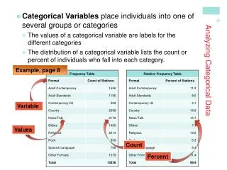
Analysing categorical variables • Frequencies • The number of observations within a given category
Assumptions of Chi squared • Each observation only contributes to only one cell of the contingency table • The expected frequencies should be greater than 5
Chi Squared II • Pearsons Chi squared • Assess the difference between observed frequencies and expected frequencies in each cell • This is achieved by calculating the expected values for each cell • Model = RT x CT N
Chi Squared III • Likelihood ratio • a comparison of observed frequencies by those predicted by the model (expected) • Yates correction • with a 2 x 2 contingency table Pearson’s chi squared can produce a type 1 error (subtract .5 from the deviation and square it) • this makes it less significant
The contingency table I • Using my case study on stop and search suppose we wanted to ascertain if black males were stopped more in one month than white males • One variable • (black or white male) • What does this tell us
One-way Chi Squared • In a simple one way chi squared we would expect that if we had 148 people they would be evenly split between white and black males so • expected values would be 78
The contingency table II • It would more useful to look at an additional variable lets say age • Two variables • Males • Black/white • Age • Under 18/over 18
Example • Now using the formula calculate the expected values for the consistency table • Model = RT x CT N
Odds ratio • The odds that a given observation is likely to happen
Loglinear analysis • Loglinear works on backward elimination of a model • Saturated first, then removes predictors • just like an ANOVA a loglinear assesses the relationship between all variables and describes the outcomes in terms of interactions
Loglinear analysis II • With our previous example we had two variables • ethnicity and age • If we now added reason for stop and search a loglinear analysis will first assess the 3-way interaction and then assess the varying two-way interactions
Assumptions of loglinear analysis • Similar to those of chi squared • observations should fall into one category alone • no more than 20% of cells with frequencies less than 5 • all cells must have frequencies greater than 1 • if you don’t meet this assumption you need to decide whether to proceed with the analysis or collapse the data across variables
Output I • No of cases should equal the no of total observations • No of factors (variables) • No of levels (sub-divisions within each variable) • Saturated model the maximum interaction possible with observed frequencies • Goodness of fit and likelihood ration statistics • the expected frequencies are significantly different from the observed • these should be non significant if model is a good fit
Output II • Goodness fit preferred for large samples • Likelihood ration is preferred for small samples • K-way higher order is asking • if you remove the highest order interaction will the fit of the model be affected • the next k-way affect asking if you remove the highest order following by the next order will the fit of the model be affected • and so on until all affects are removed
Output III • K-way effects are zero asks the opposite • that is whether removing main effects will have an effect on the model • the final step is the backward elimination • the analysis will keep going until it has eliminated all effects and advises that • the best model has generated class