Understanding Basic Statistical Concepts: From Populations to Linear Regression
This comprehensive review covers essential statistical methods, including population vs. samples, types of variables, data representation (frequency distribution, graphs), and summary statistics like measures of central tendency (mean, median) and variation (standard deviation, range). Additionally, it explores the relationships between numerical variables using correlation coefficients and linear regression techniques. Practical examples illustrate these concepts in business, economics, and the physical sciences, emphasizing prediction and data analysis through scatter plots and least-squares methodology.

Understanding Basic Statistical Concepts: From Populations to Linear Regression
E N D
Presentation Transcript
STAT 203 Elementary Statistical Methods
Review of Basic Concepts • Population and Samples • Variables and Data • Data Representation (Frequency Distn Tables, Graphs and Charts) • Descriptive Measures • Measures of Central Tendency (mean, median) • Measures of Variation(standard deviation, range etc) • Five Number Summaries AA-K 2014/15
Examining Relationships of Two Numerical Variables • In many applications, we are not only interested in understanding variables of themselves, but also interested in examining the relationships among variables. • Predictions are always required in business, economics and the physical sciences from historical or available data AA-K 2014/15
Examples • Final Exam Score, Study time and class attendance • Production; overhead cost, level of production, and the number of workers • Real Estate; value of a home, size(square feet), area • Economics; Demand and supply • Business; Dividend yield and Earnings per share AA-K 2014/15
Terminology • Dependent Variable (response variable or y-variable) • Independent Variable (predictor variable or x-variable): AA-K 2014/15
Graphical • Scatter plots (Useful for 2variables ) A scatter plot is a graph of plotted data pairs x and y. • Matrix plot (Useful for more than 2 variables) It presents the individual scatter plots in a form of a matrix AA-K 2014/15
Example • Consider some historic data for a production plant: Production Units (In 10,000s): 5 6 7 8 9 10 11 Overhead Costs (In $1000s): 12 11.5 14 15 15.4 15.3 17.5 Construct a scatter plot for y verses x AA-K 2014/15
Example (cont) AA-K 2014/15
Example of a matrix plot AA-K 2014/15
Linear Correlation Coefficient (r) • Used as a computational approach to determine the relationship between 2 variables • Pearson’s product moment correlation coefficient (PPMC) • Spearman’s rank correlation coefficient • Kendall’s correlation coefficient (τ) AA-K 2014/15
Pearson’s product moment correlation coefficient (PPMC) • Computational Formula AA-K 2014/15
Properties of the Correlation Coefficient • When , Then a perfect linear relationship exists between X and Y • When Then no linear relationship exists between X and Y • When then a weak positive linear relationship between X and Y AA-K 2014/15
Properties of the Correlation Coefficient (cont) • When then a weak negative linear relationship between X and Y • When then a strong positive linear relationship between X and Y • When then a strong positive linear relationship between X and Y AA-K 2014/15
Some scatter plots AA-K 2014/15
NOTE • The correlation only measures “linear” relationship. Therefore, when the correlation is close to 0, it indicates that the two variables have a very weak linear relationship. It does not mean that the two variables may not be related in some different functional form (like quadratic, cubic, S-shaped, etc.) AA-K 2014/15
Example of a quadratic relationship between X and Y AA-K 2014/15
Simple Linear Regression • Linear regression is a statistical technique used to describe the relationship between variables • Where the interest is to examine the relationship between 2 variables, it is referred to as Simple Linear regression (SLR) • If the relationship is believed to be linear, then the equation expressing this relationship is the equation of the line: AA-K 2014/15
Simple Linear Regression • If a graph of all the (x ,y ) pairs is plotted, and a line is determined to fit the data, then represents the y-intercept and represents the slope of the line AA-K 2014/15
Exact (Deterministic) Relationship • We do not require regression analysis to obtain the linear equation expressing an exact relation. • Exact linear relationships are encountered in some business environments For Example; AA-K 2014/15
Graph of an Exact Linear relationship AA-K 2014/15
Non-exact relationship • Data encountered in real life and many business applications do not have an exact relationship. • Exact relationships are an exception rather than the rule • Real life data are more likely to look like the graph below; AA-K 2014/15
Graph of a Non-Exact Relationship AA-K 2014/15
Assumptions for SLR • There is a linear relationship (as determined) between the 2 variables from the scatter plot • The dependent values of Y are mutually independent. • For each value of x corresponding to Y-values are normally distributed • The standard deviations of the Y-values for each value of x are the same (homoscedasticity) AA-K 2014/15
Best-Fitting Line AA-K 2014/15
Least-Square Criterion • The criterion for the best-fitting line that minimizes the “sum of squared errors” is known as the Least-Squares Criterion • The best-fitted line is denoted as; Where is the predicted value and is the intercept and slope respectively computed from the least square method AA-K 2014/15
Least-Square Criterion • The difference between the actual y-value and the predicted value is called a residual and represents the error • This error is denoted as; • The line that minimizes Is referred to at the Least-square regression line AA-K 2014/15
Least Square Criterion • The computational formulas for and that minimizes is given by • or AA-K 2014/15
Interpretation of and • represents the average change in y for a unit change in x • represents the average value of y, when x=0. (NB: this only has practical meaning when 0 is in the range of values of x) AA-K 2014/15
Computation of Error Sum of Squares (SSE) • Recall: The use of the least square criterion is to the minimize error; • The line that minimizes is the LS regression line. • is referred to as the Error sum of squares. • Denoted; AA-K 2014/15
Mean Square Error (MSE) • SSE is the sum of squared deviations of each of the observed values from the fitted regression line • SSE is often referred to as the unexplained sum of squares • The Mean Square Error (MSE) is an estimate of the variance around the regression line AA-K 2014/15
Computation of Total Sum of Squares • The total variation in the response variable (y) is referred to total sum of squares • Denoted; or SST= AA-K 2014/15
Computation of Regression Sum of Squares (SSR) • The SSR measures the improvement in using the regression line rather than the sample mean to make predictions. • Denoted; or SSR= AA-K 2014/15
Regression Mean Square • The SSR which is referred to as the explained sum of squares and it measures the “explained” variation in y by the use of x. • A measure of this variation is by use of the Mean Square Regression (MSR) AA-K 2014/15
Coefficient of Determination ( • This is a value that measures the percentage of variation in y that is explained by the regression. • or • If is computed to be 0.853, then it means 85.3% of the variation in y is explained by the regression of y on x. AA-K 2014/15
Analysis of Variance (ANOVA) Definition • Analysis of variance (ANOVA) refers to the partitioning of the total variation in the dependent variable (y) into the regression and error sum of squares. AA-K 2014/15
Analysis of Variance for SLR AA-K 2014/15
Homework 1 Q1. The following data are annual disposable income (in $1000) and the total annual consumption (in $1000) for 12 families selected at random from a large metropolitan area. AA-K 2014/15
Homework 1 (cont) i. Draw a scatter plot for the data and comment on the relationship between the 2 variables ii. Calculate the correlation coefficient and comment on the relationship between the variables. iii. Fit a simple linear regression of consumptionon income for the data. iv. Interpret the least squares regression coefficient estimates in the context of the problem AA-K 2014/15
Homework 1 (cont) v. Estimate the consumption of a family whose annual income is $17000. Would you consider the prediction as an Extrapolation? Why? vi. Draw an appropriate ANOVA table for the regression of Y on X vii. Compute the coefficient of determination R-square and interpret the value. AA-K 2014/15
Homework 1 (cont) Q2 1. Hanna Properties is a real estate company which specializes in custom-home resale in Phoenix, Arizona. The following is a sample of the size (in hundreds of square feet) and price (in thousands of dollars) data for nine custom homes currently listed for sale. AA-K 2014/15
Homework 1 (cont) a) Draw a scatter plot for the data and comment on the relationship between the 2 variables b) Calculate the correlation coefficient between the size and price of custom homes at Hanna properties and comment on the relationship between the variables. c) Fit a simple linear regression of price on size for the data. d) Interpret the least squares regression coefficient estimates in the context of the problem AA-K 2014/15
Homework 1 (cont) e) Estimate the price of a custom home from Hanna Properties if the size of the home is 3200 sq. ft? Would you consider the prediction as an Extrapolation? Why? f) Draw an appropriate ANOVA table for the regression of Y on X g) Compute the coefficient of determination R-square and interpret the value. AA-K 2014/15