Introducing Bayesian Approaches to Twin Data Analysis
360 likes | 508 Vues
Introducing Bayesian Approaches to Twin Data Analysis. Lindon Eaves, VIPBG, Richmond. Boulder, March 2001. Outline. Why use a Bayesian approach? Basic concepts “BUGS” Live Demo of simple application Applications to twin data. Why Use Bayesian Approach?. Intellectually satisfying

Introducing Bayesian Approaches to Twin Data Analysis
E N D
Presentation Transcript
Introducing Bayesian Approaches to Twin Data Analysis Lindon Eaves, VIPBG, Richmond. Boulder, March 2001
Outline • Why use a Bayesian approach? • Basic concepts • “BUGS” • Live Demo of simple application • Applications to twin data
Why Use Bayesian Approach? • Intellectually satisfying • Get more information out of existing problems (distributions of model parameters, individual“genetic” scores) • Tackle problems other methods find difficult (non-linear mixed models – growth curves; GxE interaction)
Some references Gilks, W.R., Richardson, S., Spiegelhalter, D.J. (1996) Markov Chain Monte Carlo in Practice. Chapman & Hall, London. Spiegelhalter, D., Thomas, A., Best, N. (2000) WinBUGS Version 1.3, User Manual, MRC BUGS Project: Cambridge. Eaves, L.J., Erkanli, A. (In preparation) Markov Chain Monte Carlo Approaches to Analysis of Genetic and Environmental Components of Human Developmental Change and GxE Interaction. (For Behavior Genetics).
The Traditional Approach:Via Likelihood Given Data D and parametersq: The likelihood function, l, is l=P(D|q). We find qthat maximizes l.
Typically Maximize likelihood numerically Fairly easy for linear models and normal variables (“LISREL”) Mx works well (best!)
BUT…. Some things don’t work so well
For example: • Getting confidence intervals etc. • Non-linear models (require integration over latent variables – hard for large # of parameters) • Estimating large numbers of latent variables (e.g. “genetic factor scores”)
Markov Chain Monte Carlo Methods:(MCMC) • Allow more general models • Obtain confidence intervals and other summary statistics • Estimates missing values • Estimates latent trait values All as part of the model-fitting process
Bayesian approach ML works with l=P(D|q). Bayesian approach seeks distribution of parameters given data: B=P(q|D).
How do we get P(q|D)? Use Bayes theorem: P(q|D)=P( q & D)/P(D) = P(D|q).P(q)/P(D)
A couple of problems • We don’t know P(q) • What is P(D)?
P(q) “Prior” distribution not known but may know (guess?) its form, e.g., Means may be normal Variances may be gamma
P(D) P(D)=SP(D|q).P(q)dq Where S=integral sign (!)
How do we get integral? If we know P(q) we could sample q many times and evaluate function. Integral is approximated to desired accuracy by mean of k (=large) samples (“Monte Carlo” integration)
We still have a problem.. We don’t know P(q) We only know its “shape”
“Markov Chain” Monte Carlo… Simulate a sequence of samples of q that ultimately converge to (non-independent) samples from the desired distribution, P(q).
If we succeed… When the sequence has converged (“stationary distribution”, after “burn in” from trial q) we may construct P(q) from sequence of samples.
One algorithm that can generate chains in large number of cases… …The “Gibbs Sampler”, hence: “Bayesian Inference Using Gibbs Sampling” “BUGS” for short Spiegelhalter, D., Thomas, A., Best, N. (2000) WinBUGS Version 1.3, User Manual, MRC BUGS Project: Cambridge.
Obtaining WinBUGS • Find MRC BUGS project on www (search on WinBUGS) • Download educational version (free) • Register by email (at site) • Install educational version (Instructions at site) • Follow instructions in reply email to convert to production version (free)
Preview of example: Using BUGS to estimate a mean and variance
list(n=50)y[] 14.1110 9.5125 13.2752 10.5952 8.6699... 10.0673 10.7618 8.2337 9.2170 7.3803 8.9194 4.9589list(mu=10,tau=0.2) Data and Initial Values for Mean-Variance Problem
Values of Mean (mu): First 200 iterations of MCMC Algorithm
Values of Variance (Sigma2): First 200 iterations of MCMC Algorithm
MCMC Estimates of Mean and Variance: 5000 iterations after 1000 iteration “burn in”.
Application to Twin Data Fitting the AE model to bivariate twin data
Parameter ML estimate Population value mu[1] 9.993 10.0 mu[2] 10.047 10.0 sigma2.g[1,1] 0.704 0.8 sigma2.g[1,2] 0.371 0.4 sigma2.g[2,2] 0.741 0.8 sigma2.e[1,1] 0.194 0.2 sigma2.e[1,2] 0.098 0.1 sigma2.e[2,2] 0.254 0.2 Table 1: Population parameter values used in simulation of bivariate twin data and values realized using Mx for ML estimation (N=100 MZ and 100 DZ pairs).
list(N=2,nmz=100,ndz=100,mean=c(0,0),precis =structure(.Data=c(0.0001,0, 0, 0.0001),.Dim=c(2,2)),omega.g=structure(.Data=c(0.0001,0,0,0.0001),.Dim=c(2,2)),omega.e=structure(.Data=c(0.0001,0,0,0.0001),.Dim=c(2,2)))ymz[,1,1] ymz[,1,2] ymz[,2,1] ymz[,2,2] 9.9648 9.4397 10.1008 9.6549 8.9251 10.5722 9.5299 10.5583 10.7032 9.9130 11.1373 10.2855 10.8231 11.5187 11.0396 10.7342 11.3261 12.4088 11.4504 11.9600 9.4009 10.7828 9.5653 11.8201 Start of Data for Bivariate Twin Example
Summary statistics for 5000 MCMC iterations of bivariate AE model after 2000 iteration "burn in" node mean sd MC error 2.5% median 97.5% deviance 985.7 67.7 2.91 856.7 985.4 1118.0 mu[1] 9.991 0.05906 0.001452 9.877 9.992 10.11 mu[2] 10.05 0.06184 0.001871 9.924 10.05 10.17 g[1,1] 0.705 0.08122 0.003302 0.5567 0.7018 0.8731 g[1,2] 0.3719 0.06418 0.0024 0.252 0.3711 0.5065 g[2,2] 0.7394 0.08337 0.002786 0.5885 0.7367 0.9113 e[1,1] 0.197 0.02872 0.001223 0.1476 0.1943 0.2606 e[1,2] 0.09904 0.02398 9.144E-4 0.05537 0.09788 0.1486 e[2,2] 0.2581 0.03528 0.00123 0.1977 0.2555 0.3337
Illustrative MCMC estimates of genetic effects: first two DZ twin pairs on two variables Observation Est S.e. MC error 2.5% Median 97.5% g1dz[1,1,1] 11.53 0.3756 0.007243 10.77 11.53 12.27 g1dz[1,1,2] 10.94 0.4263 0.007021 10.1 10.94 11.78 g1dz[1,2,1] 11.44 0.3763 0.006501 10.7 11.43 12.18 g1dz[1,2,2] 10.93 0.4286 0.007602 10.08 10.95 11.76 g1dz[2,1,1] 9.231 0.3776 0.007866 8.499 9.228 9.992 g1dz[2,1,2] 10.25 0.4248 0.007331 9.409 10.25 11.09 g1dz[2,2,1] 9.331 0.373 0.005969 8.606 9.329 10.07 g1dz[2,2,2] 9.505 0.4188 0.007975 8.694 9.5 10.31