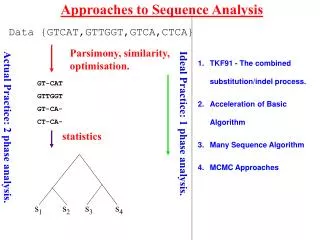
Approaches to Sequence Analysis
410 likes | 447 Vues
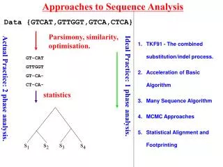
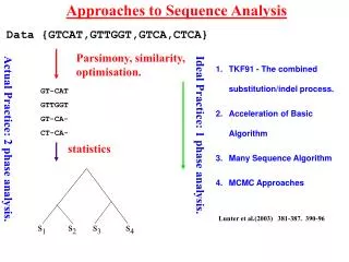
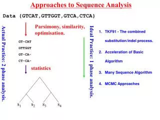
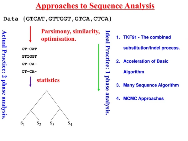
Explore sequence analysis methodologies including parsimony, similarity, and optimization techniques for DNA sequences GT-CAT, GTTGGT, GT-CA, and CT-CA. Understand ideal vs. actual practices, statistics, and algorithms like TKF91. Analyze alignments and applications in phylogeny studies.

Approaches to Sequence Analysis
E N D
Presentation Transcript
Approaches to Sequence Analysis Data {GTCAT,GTTGGT,GTCA,CTCA} Parsimony, similarity, optimisation. GT-CAT GTTGGT GT-CA- CT-CA- Ideal Practice: 1 phase analysis. Actual Practice: 2 phase analysis. statistics s1 s2 s3 s4 • TKF91 - The combined substitution/indel process. • Acceleration of Basic Algorithm • Many Sequence Algorithm • MCMC Approaches
Number of alignments, T(n,m) 1 9 41 129 321 681 T 1 7 25 63 129 231 G 1 5 13 25 41 61 T 1 3 5 7 9 11 T 1 1 1 1 1 1 C T A G G Alignments columns are equivalent to step (0,1), (1,0) and (1,1) in a [0,n][0,m] matrix. T(n,m) is the number of alignments of s1[1,n] and s2[1,m] then T(n,m)=T(n-1,m)+T(n,m-1)+T(n-1,m-1) T(0,0)=1 T(n,m) > 3 min(n,m) Thus alignment by alignment search for best alignment is not realistic. -n n- n- -n is equivalent to If then alignments are equivalent to choosing two subsets of s1 and and s2 that has to be matched, thus
Parsimony Alignment of two strings. Sequences: s1=CTAGG s2=TTGT. 5, indels (g) 10. Basic operations: transitions 2 (C-T & A-G), transversions 5, indels (g) 10. CTAG CTA G = + TT-G TT- G Cost Additivity {CTA,TT}AL + GG (A) 0 12 Min [ ] {CTA,TTG}AL + G- (B) {CTAG,TTG}AL = 10 4 12 {CTAG,TT}AL + -G (C) 10 32 Di,j=min{Di-1,j-1 + d(s1[i],s2[j]), Di,j-1 + g, Di-1,j +g} Initial condition: D0,0=0. (Di,j := D(s1[1:i], s2[1:j]))
T G T T C T A G G 40 32 22 14 9 17 30 22 12 4 22 20 12 212 22 32 10 2 10 20 30 40 10 20 30 40 50 12 0 CTAGG Alignment: i v Cost 17 TT-GT
Alignment of three sequences. A C ? A s1=ATCG s2=ATGCC s3=CTCC A A C Alignment: AT-CG ATGCC CT-CC Consensus sequence: ATCC Configurations in an alignment column: - - n n n - n - - n - n - n n - n - - - n n n - Recursion:Di,j,k = min{Di-i',j-j',k-k' + d(i,i',j,j',k,k')} Initial condition: D0,0,0 = 0. Running time: l1*l2*l3*(23-1) Memory requirement: l1*l2*l3 New phenomena: ancestral/consensus sequence.
Parsimony Alignment of four sequences C G G C s1=ATCG s2=ATGCC s3=CTCC s4=ACGCG Alignment: AT-CG ATGCC CT-CC ACGCG G C C G Configurations in alignment columns: - - - n - - - n n n - n n n n - - - n - n n - n - - n - n n n - - n - - n - n - n - n n - n n - n - - - - n n - - n n n n - n - Recursion:Di= min{Di-∆ + d(i,∆)} ∆ [{0,1}4\{0}4] Initial condition: D0 = 0.Memory : l1*l2*l3*l4 Computation time: l1*l2*l3*l4*24Memory : l1*l2*l3*l4 New Phenomena: Cost and alignment is phylogeny dependent
Progressive Alignment (Feng-Doolittle 1987 J.Mol.Evol.) Can align alignments and given a tree make a multiple alignment. * * alkmny-trwq acdeqrt akkmdyftrwq acdehrt kkkmemftrwq [ P(n,q) + P(n,h) + P(d,q) + P(d,h) + P(e,q) + P(e,h)]/6 * * *** * * * * * * Sodh atkavcvlkgdgpqvqgsinfeqkesdgpvkvwgsikglte-glhgfhvhqfg----ndtagct sagphfnp lsrk Sodb atkavcvlkgdgpqvqgtinfeak-gdtvkvwgsikglte—-glhgfhvhqfg----ndtagct sagphfnp lsrk Sodl atkavcvlkgdgpqvqgsinfeqkesdgpvkvwgsikglte-glhgfhvhqfg----ndtagct sagphfnp lsrk Sddm atkavcvlkgdgpqvq -infeak-gdtvkvwgsikglte—-glhgfhvhqfg----ndtagct sagphfnp lsrk Sdmz atkavcvlkgdgpqvq— infeqkesdgpvkvwgsikglte—glhgfhvhqfg----ndtagct sagphfnp Lsrk Sods vatkavcvlkgdgpqvq— infeak-gdtvkvwgsikgltepnglhgfhvhqfg----ndtagct sagphfnp lsrk Sdpb datkavcvlkgdgpqvq—-infeqkesdgpv----wgsikgltglhgfhvhqfgscasndtagctvlggssagphfnpehtnk sddm Sodb Sodl Sodh Sdmz sods Sdpb
T= 0 # - - - ## # # # T = t # # # # s1 r s2 s1 s2 s1 s2 Thorne-Kishino-Felsenstein (1991) Process A # C G * • (birth rate) < m(death rate) 1. P(s) = (1-l/m)(l/m)l pA#A* .. *pT #T l =length(s) 2. Time reversible:
# - - - - - # # # # k * - - - - * # # # # k l & m into Alignment Blocks A. Amino Acids Ignored: # - - - ## # # k e-mt[1-lb](lb)k-1 [1-lb-mb](lb)k [1-lb](lb)k p’k(t) pk(t) p’’k(t) b=[1-e(l-m)t]/[m-le(l-m)t] p’0(t)= mb(t) B. Amino Acids Considered: T - - - RQ S W Pt(T-->R)*pQ*..*pW*p4(t) 4 T - - - - • R Q S WpR *pQ*..*pW*p’4(t) 4
Basic Pairwise Recursion (O(length3)) i j Survives: Dies: i-1 i i-1 i j-1 j j i-1 i i j-2 j i-1 j j-1 …………………… …………………… …………………… e-mt[1-lb](lb)k-1, where …………………… …………………… b=[1-e(l-m)t]/[m-le(l-m)t] 0… j (j+1) cases 1… j (j) cases
Basic Pairwise Recursion (O(length3)) survive death j (i-1,j) j-1 (i-1,j-1) Initial condition: p’’=s2[1:j] ………….. (i-1,j-k) ………….. ………….. i-1 i (i,j)
Corner Cutting ~100-1000 Better Numerical Search ~10-100 Ex.: good start guess, 28 evaluations, 3 iterations Accelleration of Pairwise Algorithm (From Hein,Wiuf,Knudsen,Moeller & Wiebling 2000) Simpler Recursion ~3-10 Faster Computers ~250 1991-->2000 ~106
a-globin (141) and b-globin (146) (From Hein,Wiuf,Knudsen,Moeller & Wiebling 2000) 430.108 : -log(a-globin) 327.320 : -log(a-globin -->b-globin) 747.428 : -log(a-globin, b-globin) = -log(l(sumalign)) l*t: 0.0371805 +/- 0.0135899 m*t: 0.0374396 +/- 0.0136846 s*t: 0.91701 +/- 0.119556 E(Length) E(Insertions,Deletions) E(Substitutions) 143.499 5.37255 131.59 Maximum contributing alignment: V-LSPADKTNVKAAWGKVGAHAGEYGAEALERMFLSFPTTKTYFPHF-DLS--H---GSAQVKGHGKKVADALT VHLTPEEKSAVTALWGKV--NVDEVGGEALGRLLVVYPWTQRFFESFGDLSTPDAVMGNPKVKAHGKKVLGAFS NAVAHVDDMPNALSALSDLHAHKLRVDPVNFKLLSHCLLVTLAAHLPAEFTPAVHASLDKFLASVSTVLTSKYR DGLAHLDNLKGTFATLSELHCDKLHVDPENFRLLGNVLVCVLAHHFGKEFTPPVQAAYQKVVAGVANALAHKYH Ratio l(maxalign)/l(sumalign) = 0.00565064
Homology test. (From Hein,Wiuf,Knudsen,Moeller & Wiebling 2000) Real s1 = ATWYFCAK-AC s2 = ETWYKCALLAD *** ** * Wi,j= -ln(pi*P2.5i,j/(pi*pj)) D(s1,s2) is evaluated in D(s1,s2*) a-, myoglobin homology tests Random s1 = ATWYFC-AKAC s2* = LTAYKADCWLE * 1. Test the competing hypothesis that 2 sequences are 2.5 events apart versus infinitely far apart. 2. It only handles substitutions “correctly”. The rationale for indel costs are more arbitrary.
Sample random alignments from real sequences Sample random alignments from random sequences cgtgttacatatatatagccgatagccg cgtgttacatatatatagccgatagccg cgtgttacatatatatagccgatagccg cgtgttacatatatatagccgatagccg Compare real and random distribution using Chi-square statistic. Goodness-of-fit of TKF91
Algorithm for alignment on star tree (O(length6))(Steel & Hein, 2001) *ACGC *TT GT s2 s1 a s3 *ACG GT *###### * (l/m)
Statistical Alignment via Hidden Markov Models Steel and Hein,2001 + Holmes and Bruno,2001 - # # E # # - E * * lb l/m (1- lb)e-m l/m (1- lb)(1- e-m) (1- l/m) (1- lb) - # lb l/m (1- lb)e-m l/m (1- lb)(1- e-m) (1- l/m) (1- lb) # #lb l/m (1- lb)e-m l/m (1- lb)(1- e-m) (1- l/m) (1- lb) # - lb HMM formulation allows: p(C)f(CT) T Finding most probable alignment p(A) Probability of sequence pair l/m (1- lb)(1-e-m) p(C)f(CC) C l/m (1- lb)e-m Probability of specific edge C A C
Transition Probabilities between two k-ancestral states 0 #- 1 -- 2 #- 3 ## 4 -# 5 ## 6 #- 7 # - 1 4 0 # - 5 2 3 6 7
Maximum likelihood phylogeny and alignment Gerton Lunter Istvan Miklos Alexei Drummond Yun Song Human alpha hemoglobin;Human beta hemoglobin; Human myoglobin Bean leghemoglobin Probability of data e-1560.138 Probability of data and alignment e-1593.223 Probability of alignment given data 4.279 * 10-15 = e-33.085 Ratio of insertion-deletions to substitutions: 0.0334
The phylogeny moves: As in Drummond et al. 2002 Metropolis-Hastings Statistical Alignment. Lunter, Drummond, Miklos, Jensen & Hein, 2005 The alignment moves: QST--QCC-S S------CCS ---QST--QC ---QST--QC TNQHVSCTGN GN-HVSCTGK TNQH-SCTLN TNQHVSCTLN ALITL---GG ALLTLTTLGG ---TLTSLGA ALLGLTSLGA We choose a random window in the current alignment Then delete all gaps so we get back subsequences QSTQCCS SCCS QSTQC QSTQC TNQHVSCTGN GN-HVSCTGK TNQH-SCTLN TNQHVSCTLN ALITL---GG ALLTLTTLGG ---TLTSLGA ALLGLTSLGA QSTQCCS -S--CCS QSTQC-- QSTQC-- TNQHVSCTGN GN-HVSCTGK TNQH-SCTLN TNQHVSCTLN ALITL---GG ALLTLTTLGG ---TLTSLGA ALLGLTSLGA Stochastically realign this part
Metropolis-Hastings Statistical Alignment Lunter, Drummond, Miklos, Jensen & Hein, 2005
Many Sequences: Sequence Graphs (reticular alignment) Istvan Miklos – Gerton Lunter – Miklos Csuros Investigate a set of ancestral sequences/alignments that are computationally realistic • A set of homologous sequences are given • With a known phylogeny • Pairs of sequences are aligned • Graphs defined representing alignment/ancestral sequences • Pairs of graphs aligned…. ccgttagct ccgttagct ccgttagct ccgttagct
Extensions • TKF92 Like TKF91, except that that nucleotides are substituted by geometric length flakes of nucleotides. A flake does not experience indels. • Long Indel Model Now the insertions will have to be given a length distribution. Deletions will be associated intervals on the sequences. An l4 algorithm is available. # # # # # • Local Statistical Alignment Homologous segments are now embedded with unrelated sequences. Both regions can be well modelled.
Summary and Future Work A statistical approach to alignment • A Stochastic Model including Insertion-Deletions • The fate of a single nucleotide • Dynamical Programming solution to the pairwise problem • An HMM solution to pairwise statistical alignment • Multiple statistical alignment Problems Ahead (enough to do) • Longer Insertion-Deletions • Heterogeneity of positions • Testing Models • Combining with Annotation • Very Large Number of Sequences
References Statistical Alignment • Fleissner R, Metzler D, von Haeseler A.Simultaneous statistical multiple alignment and phylogeny reconstruction.Syst Biol. 2005 Aug;54(4):548-61. • Hein,J., C.Wiuf, B.Knudsen, Møller, M., and G.Wibling (2000): Statistical Alignment: Computational Properties, Homology Testing and Goodness-of-Fit. (J. Molecular Biology 302.265-279) • Hein,J.J. (2001): A generalisation of the Thorne-Kishino-Felsenstein model of Statistical Alignment to k sequences related by a binary tree. (Pac.Symp.Biocompu. 2001 p179-190 (eds RB Altman et al.) • Steel, M. & J.J.Hein (2001): A generalisation of the Thorne-Kishino-Felsenstein model of Statistical Alignment to k sequences related by a star tree. ( Letters in Applied Mathematics) • Hein JJ, J.L.Jensen, C.Pedersen (2002) Algorithms for Multiple Statistical Alignment. (PNAS) 2003 Dec 9;100(25):14960-5. • • Holmes, I. (2003) Using Guide Trees to Construct Multiple-Sequence Evolutionary HMMs.Bioinformatics, special issue for ISMB2003, 19:147i–157i. • • Jensen, J.L. & Hein, J. (2004) A Gibbs sampler for statistical multiple alignment. Statistica Sinica, in press. • • Miklós, I., Lunter, G.A. & Holmes, I. (2004) A 'long indel' model for evolutionary sequence alignment. Mol. Biol. Evol. 21(3):529–540. • • Lunter, G.A., Miklós, I., Drummond, A.J., Jensen, J.L. & Hein, J. (2005) Bayesian Coestimation of Phylogeny and Sequence Alignment. BMC Bioinformatics, 6:83 • • Lunter, G.A., Miklós, I., Drummond, A., Jensen, J.L. & Hein, J. (2003) Bayesian phylogenetic inference under a statistical indel model. pspdfLecture Notes in Bioinformatics, Proceedings of WABI'03, 2812:228–244. • • Lunter, G.A., Miklós, I., Song, Y.S. & Hein, J (2003) An efficient algorithm for statistical multiple alignment on arbitrary phylogenetic trees.J. Comp. Biol., 10(6):869–88Miklos, Lunter & Holmes (2002) (submitted ISMB) • Miklos, I & Toroczkai Z. (2001) An improved model for statistical alignment, in WABI2001, Lecture Notes in Computer Science, (O. Gascuel & BME Moret, eds) 2149:1-10. Springer, Berlin • Metzler D. “Statistical alignment based on fragment insertion and deletion models.” Bioinformatics. 2003 Mar 1;19(4):490-9. • Miklos, I (2002) An improved algorithm for statistical alignment of sequences related by a star tree. Bul. Math. Biol. 64:771-779. • Miklos, I: Algorithm for statistical alignment of sequences derived from a Poisson sequence length distribution Disc. Appl. Math. accepted. • Thorne JL, Kishino H, Felsenstein J.Inching toward reality: an improved likelihood model of sequence evolution.J Mol Evol. 1992 Jan;34(1):3-16. • Thorne JL, Kishino H, Felsenstein J.An evolutionary model for maximum likelihood alignment of DNA sequences.J Mol Evol. 1991 Aug;33(2):114-24. Erratum in: J Mol Evol 1992 Jan;34(1):91. • Thorne JL, Churchill GA.Estimation and reliability of molecular sequence alignments.Biometrics. 1995 Mar;51(1):100-13. TKF92, Long Indel, Explain HMM, Multiple Recursion, Hidden State Space, 1-state recursion and other reductions, competing algorithms,
VLSPADNAL.....DLHAHKR 141 AA long *########### …. ### 141 AA long 2 108 years 2 107 years 2 109 years *########### …. ### *########### …. ### ???????????????????? k AA long 109 years The invasion of the immortal link
Binary Tree Problem a1a2 * * # # # - - # # # - # TGA ACCT s1 s3 a1 a2 s2 s4 GTT ACG • The ancestral sequences & their alignment was known. ii. The alignment of ancestral alignment columns to leaf sequences was known The problem would be simpler if: How to sum over all possible ancestral sequences and their alignments?: A Markov chain generating ancestral alignments can solve the problem!!
One block derivation # - - ... - # #*# ... # 1 k-1 # - - ... - # # # ... # 1 k+1 # - - ... - # # # ... # 1 k pk # - - ... - # #*# ... # 1 k-1 # - - ... - # # # ... # 1 k+1 Dpk = Dt*[l*(k-1) pk-1 + m*k*pk+1 - (l+m)*k*pk]
Dpk = Dt*[l*(k-1) pk-1 + m*k*pk+1 - (l+m)*k*pk] Dp’k=Dt*[l*(k-1) p’k-1+m*(k+1)*p’k+1-(l+m)*k*p’k+m*pk+1] Dp’’k=Dt*[l*k*p’’k-1+m*(k+1)*p’’k+1- [(k+1)l+km]*p’’k] Differential Equations for p-functions # - - ... - # # # ... # # - - - ... - - # # # ... # * - - - ... - * # # # ... # Initial Conditions: pk(0)= pk’’(0)= p’k (0)= 0 k>1 p1(0)= p0’’(0)= 1. p’0 (0)= 0
TKF92 - Unbreakable fragments • Fragments evolve into fragments. • All possible tilings of the sequences with geometric length fragments are considered.
Long Insertion-Deletions can model overlapping indels more involved dynamic programming:
Many un-aligned sequences related by a known phylogeny: • Conceptually simple, computationally hard • Dependent on a single alignment/no measure of uncertainty • Statistical Alignment • Explicit stochastic model of substitution and indel evolution A C sometimes - # # # # - HMM: A T G • Advantages: Summing over uncertainty + confidence on inference The Basics of Footprinting II
Statistical Alignment andFootprinting. acgtttgaaccgag---- 1 acgtttgaaccgag---- sequences sequences 1 k k Comment:The A-HMM * S-HMM is an approximate approach as S-HMM does not include an evolutionary model acgtttgaaccgag---- 1 sequences Alignment HMM k Ex.: nnnnnnnnnnn Alignment HMM Signal HMM nnnnnnnnnnn
Structure HMM S F F F S S 0.1 0.1 0.1 0.1 0.9 0.9 F S SF FS SS FF (A,S) F F S S F Alignment HMM ? Structure HMM “Structure” does not stem from an evolutionary model • The equilibrium annotation does not follow a Markov Chain: • Each alignment in from theAlignment HMM is annotated by the Structure HMM: • No ideal way of simulating: using the HMM at the alignment will give other distributions on the leaves using the HMM at the root will give other distributions on the leaves
Ancestral Sequence Generator # E * l/m 1- l/m #l/m 1- l/m * # # # # p’’ function generator - # E * - - - - * # # # # lb 1- lb lb 1- lb * * - # p’/p function generator # - - - - # # # # # - # E lb 1- lb 1-mb mb # # # - # - - - - - # # # # lb 1- lb - # Markov Chains Generating the p-functions
The Basic Recursion ”Remove 1st step” - recursion: S E ”Remove last step” - recursion: Last/First step removal are inequivalent, but have the same complexities. First step algorithm is the simplest.
Sequence Recursion: First Step Removal Pa(Sk): Epifixes (S[k+1:l]) starting in given MC starts in a. Pa(Sk) = e a E Where P’(kS i,H) = F(kSi,H)
Fundamental Pairwise Recursion. P(s1i->s2j) = p’0P(s1i-1->s2j) + Initial Condition P(s10 ->s2j) = pj’’ps2[1:j] Simplification: Ri,j =(p1f(s1[i],s2[j]+p’1ps2j[j])P(s1i-1->s2j-1) P(s1i->s2j) = Ri,j + p’0 P(s1i->s2j-1) P(s1i->s2j) = p’0P(s1i-1->s2j)+ lbP(s1i->s2j-1) + (p1f(s1[i],s2[j]+p’1ps2j[j]- lb ps2j[j] ))P(s1i-1->s2j-1) Probability of observation P(s1 , s2) = P(s1) P(s1 ->s2)
Gibbs Samplers for Statistical Alignment Holmes & Bruno (2001): Sampling Ancestors to pairs. Jensen & Hein (in press): Sampling nodes adjacent to triples Slower basic operation, faster mixing
Statistical Alignment, Homology and Linguistics https://www.stats.ox.ac.uk/research/genome/projects/pastprojects • String Comparison • String Homology Robin Ryder 2008 Markus Gerstel Stephen Clark
Refinements to Statistical Alignment The present model of statistical alignment is very naive. Much is needed for both biological and linguistics applications. Here is a short list. ATWYFCAKAC 1. Longer insertion-deletions A--YFCAKAC ATWYFCAKAC 2. Swaps ATWYCFAKAC 3.Positional heterogeneity/ Functional annotation/Hidden States FFFSSFSSSS ATWYFCAKAC 4. Long Distance Correlations 5. Better equilibrium distribution