Advances in Data Analysis Approaches: Parsimony, Similarity, and Statistical Alignment Methods
This document delves into contemporary methodologies for data analysis, focusing on parsimony, similarity, and optimization techniques, primarily within the context of statistical alignment. It explores the historical foundations laid by Bishop & Thompson (1986) and Thorne et al. (1991) while addressing significant challenges faced in statistical alignment. The analysis includes the implications of phylogenetic relationships and molecular evolution, presenting various models for multiple sequence alignments and the computation of likelihood surfaces for biological data.

Advances in Data Analysis Approaches: Parsimony, Similarity, and Statistical Alignment Methods
E N D
Presentation Transcript
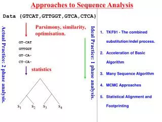
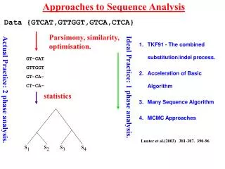
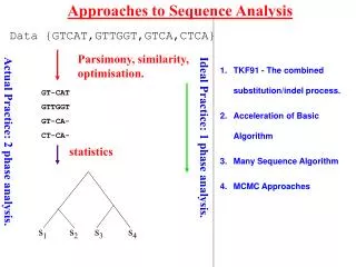
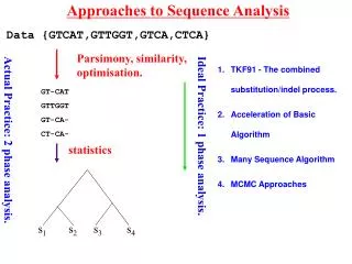
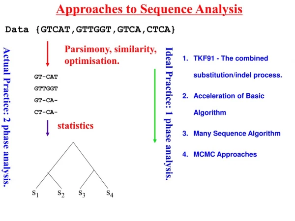
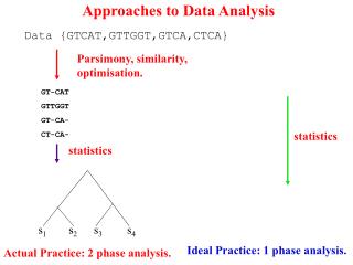
Approaches to Data Analysis s1 s2 s3 s4 Data {GTCAT,GTTGGT,GTCA,CTCA} Parsimony, similarity, optimisation. GT-CAT GTTGGT GT-CA- CT-CA- statistics statistics Ideal Practice: 1 phase analysis. Actual Practice: 2 phase analysis.
Origins of Statistical Alignment Bishop & Thompson 1986 Thorne Kishino & Felsenstein 1991 Challenges to Statistical Alignment Understanding the Basic Model Speed of the Basic Algorithm Analyzing Many Sequences - Multiple Statistical Alignment Realistic Models The Biological Problems Phylogeny & Molecular Evolution Alignment Homology Testing + More
Thorne-Kishino-Felsenstein (1991) Process * A # C G T= 0 # - - - ## # # # T = t # # # # l < m P(s) = (1-l/m)(l/m)l pA#A* .. *pT #T l =length(s) Time reversible
The invasion of the immortal link (From Hein,Wiuf,Knudsen,Moeller & Wiebling 2000)
Time reversibility Pi,j(t) = probability that i has evolved into j after time t. p(i) = probability of i after infinitely long time - equilibrium distribution p(i) Pi,j(t) = p(j) Pj,i(t) a t1 t2 s2 s1 s1 s2 t1 +t2
Two kinds of alignment Optimisation (here Parsimony): Shortest Path C T G A G G G T - - G C CTGAGG GTGC Statistical: Probability and Sum over all Paths C T G A G G G T - - G C CTGAGG GTGC
l & m into Alignment Blocks A. Amino Acids Ignored: # - - - # - - - - * - - - - ## # # - # # # # * # # # # k k k e-mt[1-lb(t)](lb(t))k-1 [1-e-mt-mb(t)][1-lb(t)](lb(t))k-1 [1-lb(t)](lb(t))k pk(t) p’k(t) p’’k(t) p’0(t)= mb(t) b(t)=[1-e(l-m)t]/[m-l] B. Amino Acids Considered: T - - - RQ S W Pt(T-->R)*pQ*..*pW*p4(t) 4 T - - - - - R Q S WpR *pQ*..*pW*p’4(t)
Illustration of single equation. # - - ... - # # # ... # pk+1 m # - - ... - - # # ... # p’k m*k l*k l*(k-1) m*(k+1) # - ... - - # ... # # - - - ... - - # # # ... # p’k+1 p’k-1 Dp’k=Dt*[l*(k-1) p’k-1+m*(k+1)*p’k+1 -(l+m)*k*p’k+m*pk+1]
Diff. Equations for p-functions # - - ... - # # # ... # Dpk = Dt*[l*(k-1) pk-1 + m*k*pk+1 - (l+m)*k*pk] # - - - ... - - # # # ... # Dp’k=Dt*[l*(k-1) p’k-1+m*(k+1)*p’k+1-(l+m)*k*p’k+m*pk+1] * - - - ... - * # # # ... # Dp’’k=Dt*[l*k*p’’k-1+m*(k-1)*p’’k+1-((k+1)l+mk)*p’’k] Initial Conditions: pk(0)= pk’’(0)= p’k (0)= 0 k>1 p0(0)= p0’’(0)= 1. p’0 (0)= 0
Basic Pairwise Recursion (O(length3)) i i-1 j j-1 i j Survives: Dies: i-1 i i-1 i j-1 j j i-1 i j-2 j …………………… …………………… …………………… …………………… …………………… …………………… 1… j (j) cases 0… j (j+1) cases
survive death Basic Pairwise Recursion (O(length3)) j (i,j) (i-1,j) j-1 (i-1,j-1) Initial condition: p’’=s2[1:j] ………….. (i-1,j-k) ………….. ………….. i-1 i
Fundamental Pairwise Recursion. P(s1i->s2j) = p’0P(s1i-1->s2j) + Initial Condition P(s10 ->s2j) = pj’’ps2[1:j] Probability of observationP(s1,s2) = P(s1) P(s1 ->s2) Simplification: Ri,j=(p1f(s1[i],s2[j])+p’1ps2j[j])P(s1i-1->s2j-1) + lb ps2[j]Ri,j-1 P(s1i->s2j) = Ri,j + p’0 P(s1i->s2j-1) P(s1i->s2j) = p’0P(s1i-1->s2j)+ lbP(s1i->s2j-1) + (p1f(s1[i],s2[j]+p’1ps2j[j]- lb ps2j[j] ))P(s1i-1->s2j-1)
Geometric Like Offspring Number # - - - # - - - - ## # # - # # # # k k e-mt[1-lb(t)](lb(t))k-1 [1-e-mt-mb(t)][1-lb(t)](lb(t))k-1 pk(t) p’k(t) p’0(t)= mb(t) Alternative traversal: Die forward in time Give birth backwards Trace leftmost unfinished branch. After one survivor, branch lengths With birth possibility always t.
Quadratic Recursion (i,j) (i-1,j) (i-1,j-1) (i,j-1) Two state recursion: Ri,j=(p1f(s1[i],s2[j])+p’1ps2j[j])P(s1i-1->s2j-1)+ lb ps2[j]Ri,j-1 P(s1i->s2j) = Ri,j + p’0 P(s1i->s2j-1) One state recursion: P(s1i->s2j) = p’0P(s1i-1->s2j)+ lbP(s1i->s2j-1) + (p1f(s1[i],s2[j]+p’1ps2j[j]- lb ps2j[j] ))P(s1i-1->s2j-1) 1. Summation, Maximization and Sampling of Alignments. 2. For more sequences: Ancestral Sequences & Alignments.
Likelihood Surface (From Hein,Wiuf,Knudsen,Moeller & Wiebling 2000)
a-globin (141) and b-globin (146) (From Hein,Wiuf,Knudsen,Moeller & Wiebling 2000) 430.108 : -log(a-globin) 327.320 : -log(a-globin -->b-globin) 730.428 : -log(a-globin, b-globin) = -log(l(sumalign)) l*t: 0.0371805 +/- 0.0135899 m*t: 0.0374396 +/- 0.0136846 s*t: 0.91701 +/- 0.119556 E(Length) E(Insertions,Deletions) E(Substitutions) 143.499 5.37255 131.59 Maximum contributing alignment: V-LSPADKTNVKAAWGKVGAHAGEYGAEALERMFLSFPTTKTYFPHF-DLS--H---GSAQVKGHGKKVADALT VHLTPEEKSAVTALWGKV--NVDEVGGEALGRLLVVYPWTQRFFESFGDLSTPDAVMGNPKVKAHGKKVLGAFS NAVAHVDDMPNALSALSDLHAHKLRVDPVNFKLLSHCLLVTLAAHLPAEFTPAVHASLDKFLASVSTVLTSKYR DGLAHLDNLKGTFATLSELHCDKLHVDPENFRLLGNVLVCVLAHHFGKEFTPPVQAAYQKVVAGVANALAHKYH Ratio l(maxalign)/l(sumalign) = 0.00565064
Likelihood Surface (From Hein,Wiuf,Knudsen,Moeller & Wiebling 2000)
Homology Test Wi,j= -ln(pi*P2.5i,j/(pi*pj)) D(s1,s2) is evaluated in D(s1,s2*) Real s1 = ATWYFCAK-AC Random s1 = ATWYFC-AKAC s2 = ETWYKCALLAD s2* = LTAYKADCWLE *** ** * * * This test: 1. Test the competing hypothesis that 2 sequences are 2.5 events apart versus infinitely far apart. 2. It only handles substitutions “correctly”. The rationale for indel costs are more arbitrary. 3. It samples in (pi*pj) by permuting the order of amino acids in the second. I.e. uses drawing without replacement – a hypergeometric distribution.
a-, myoglobin homology test (From Hein,Wiuf,Knudsen,Moeller & Wiebling 2000)
Algorithm for alignment on star tree (O(length6))(Steel & Hein, 2001) *ACGC *TT GT s2 s1 a *###### * (l/m) s3 *ACG GT
Binary Tree Problem TGA ACCT s1 s3 a1 a2 s2 s4 GTT ACG
Binary Tree Problem TGA ACCT a1a2 * * # # # - - # # # - # s1 s3 a1 a2 s2 s4 GTT ACG • The problem would be simpler if: • The ancestral sequences & their alignment was known. • ii. The alignment of ancestral alignment columns to leaf sequences was known. A markov chain generating ancestral alignments can solve the problem!!
# E * l/m 1- l/m #l/m 1- l/m - # E lb 1- lb lb 1- lb * * - # Markov Chains Generating the p-functions Ancestral Sequence Generator * # # # # p’’ function generator * - - - - * # # # # p’/p function generator # - - - - # # # # # - # E lb 1- lb 1-mb mb # # # - # - - - - - # # # # lb 1- lb - #
Generating Ancestral Alignments. - # # E # # - E * * lb l/m (1- lb)e-m l/m (1- lb)(1- e-m) (1- l/m) (1- lb) - # lb l/m (1- lb)e-m l/m (1- lb)(1- e-m) (1- l/m) (1- lb) _ #lb l/m (1- lb)e-m l/m (1- lb)(1- e-m) (1- l/m) (1- lb) # - lb a1 * - # E a2 * # # E lb l/m (1- lb)e-m (1- l/m) (1- lb)
The Basic Recursion ”Remove 1st step” - recursion: S E ”Remove last step” - recursion:
4-Sequence Recursion II: First Step Removal Pa(Sk): Epifixes (S[k+1:l]) starting in given MC starts in a. Pa(Sk) = Where P’(kS i,H) = F(kSi,H)
Example: 4 globins logLikelikelihood = -1593.223
O(lk)algorithm for k sequences s1 s3 a1 a2 s2 s4 Two Approaches: Use geometric tails of p-functions & suitable rearrangements. Make ”ancestral” Markov Chain for the leaves as well:
Contrasting Probability & Distance Recursions # # # # - # = = + Probability: O(l2k) – O(lk) possible Distance (Sankoff, 1973) - O(lk): A C - A 15 cases
k ancestral sequence Markov Chain State Space: * E # * E # All connected . , . , # & . . # #-tuples * E # # a4 - a4 - # / # # / a1 ---a2----a3 a1 ---a2----a3 # \ - \ - a5 - a5
k ancestral sequences: 2 Problems 1. Ambigous Indel/Alignment relationship. a #- / \ / \ s1 -# -# s2 s1 - # - - - # a # - - # - - s2 - - # - # - 2. Grand children before younger siblings. a # - - - - - - - - a1 # # - - - - # # # a2 - # # # # # - - -
Transition Probabilities between two k-ancestral states 0 #- 1 -- 2 #- 3 ## 4 -# 5 ## 6 #- 7 # - 1 4 0 # - 5 2 3 6 7
Gibbs Samplers for Statistical Alignment Holmes & Bruno (2001): Sampling Ancestors to pairs. Jensen & Hein (subm.): Sampling nodes adjacent to triples Slower basic operation, faster mixing
Work in Progress & Plans State Reduction (Lunter, Song, Hein & Miklos) Longer Insertion-Deletions (Miklos, Lunter, Holmes) * A TC CG * A TC CG Heterogeneity along Sequence(Skou, Hein,..) HMM/SCFG – like? TT Acceleration & Implementation (Lunter & Song) MCMC Methods (Ledet Jensen, Holmes,...........)
Statistical Alignment Summary Motivation for statistical alignment: i. Data is sequences - not alignment! ii. The focus on alignments is exagerated!! Progress Major Accelerations for pairwise/multiple statistical alignment Longer Insertion-Deletions models Challenges ahead Position Heterogeneity – hmm & scfg analogues. Algorithms for large data sets (>5 sequences) MCMC. Local alignment version Software ???
Acknowledgements (www.stats.ox.ac.uk/hein) Pairwise (with Knudsen, Wiuf, Møller, Wibling) Simpler recursion. Computational acceleration. Multiple Star Tree (with M.Steel) Binary Tree (with C.Storm, Jens Ledet, Lunter, Miklos,Song,Holmes,..) Gibbs Multiple Alignment (withJens Ledet) Articles & Manuscripts: 1. Hein,J.J., C.Wiuf, B.Knudsen, Møller, M., and G.Wibling (2000): Statistical Alignment: Computational Properties, Homology Testing and Goodness-of-Fit. (J. Molecular Biology 302.265-279) 2. J.J.Hein (2001): A generalisation of the Thorne-Kishino-Felsenstein model of Statistical Alignment to k sequences related by a binary tree. (Pac.Symp.Biocompu. 2001 p179-190 (eds RB Altman et al.) 3. Steel, M. & J.J.Hein (2001): A generalisation of the Thorne-Kishino-Felsenstein model of Statistical Alignment to k sequences related by a star tree. ( Letters in Applied Mathematics) 4. JJ Hein, J.L.Jensen, C.Pedersen (2002) Algorithms for Multiple Statistical Alignment. (submitted to PNAS) 5. J.L.Jensen & JJ Hein (2002) A Gibbs Sampler for Multiple Statistical Alignment. (submitted Statistical Journal…) 6. Lunter, Song, Miklos & Hein (2002) (In Press J.Com.Biol.) 7. Lunter, Song, & Hein (2003) (in prep.) 8. Miklos, Lunter & Holmes (2002) (in press MBE) 9. Miklos, I & Toroczkai Z. (2001) An improved model for statistical alignment, in WABI2001, Lecture Notes in Computer Science, (O. Gascuel & BME Moret, eds) 2149:1-10. Springer, Berlin 10 Miklos, I (2002) An improved algorithm for statistical alignment of sequences related by a star tree. Bul. Math. Biol. 64:771-779. 11 Miklos, I: (2002) “Algorithm for statistical alignment of sequences derived from a Poisson sequence length distribution” Disc. Appl. Math. accepted. 12 Holmes, I & W.Bruno (2001) “Evolutionary HMMs: A Bayesian Approach to Multiple Alignment ” Bioinformatics 17.9.803-20.