Download
1 / 15
150 likes | 377 Vues
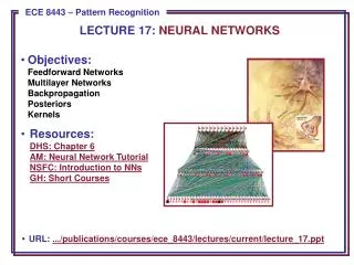
LECTURE 17: NEURAL NETWORKS. Objectives: Feedforward Networks Multilayer Networks Backpropagation Posteriors Kernels Resources: DHS: Chapter 6 AM: Neural Network Tutorial NSFC: Introduction to NNs GH: Short Courses. • URL: .../publications/courses/ece_8443/lectures/current/lecture_17.ppt.

E N D
LECTURE 17: NEURAL NETWORKS • Objectives:Feedforward NetworksMultilayer NetworksBackpropagationPosteriorsKernels • Resources:DHS: Chapter 6AM: Neural Network TutorialNSFC: Introduction to NNsGH: Short Courses • URL: .../publications/courses/ece_8443/lectures/current/lecture_17.ppt
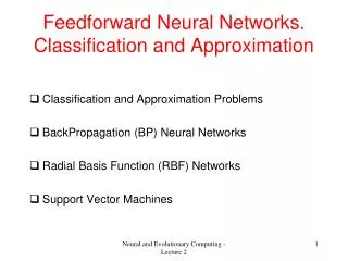
Overview • There are many problems for which linear discriminant functions are insufficient for minimum error. • Previous methods, such as Support Vector Machines require judicious choice of a kernel function (though data-driven methods to estimate kernels exist). • A “brute” approach might be to select a complete basis set such as all polynomials; such a classifier would require too many parameters to be determined from a limited number of training samples. • There is no automatic method for determining the nonlinearities when no information is provided to the classifier. • Multilayer Neural Networks attempt to learn the form of the nonlinearity from the training data. • These were loosely motivated by attempts to emulate behavior of the human brain, though the individual computation units (e.g., a node) and training procedures (e.g., backpropagation) are not intended to replicate properties of a human brain. • Learning algorithms are generally gradient-descent approaches to minimizing error.
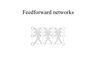
Feedforward Networks • A three-layer neural network consists of an input layer, a hidden layer and an output layer interconnected by modifiable weights represented by links between layers. • A bias term that is connected to all units. • This simple network can solve the exclusive-OR problem. • The hidden and output units from the linear weighted sum of their inputs and perform a simple thresholding (+1 if the inputs are greater than zero, -1 otherwise).
Definitions • A single “bias unit” is connected to each unit other than the input units. • Net activation: • where the subscript i indexes units in the input layer,jin the hidden; wjidenotes the input-to-hidden layer weights at the hidden unit j. • Each hidden unit emits an output that is a nonlinear function of its activation: yj= f(netj) • Even though the individual computational units are simple (e.g., a simple threshold), a collection of large numbers of simple nonlinear units can result in a powerful learning machine (similar to the human brain). • Each output unit similarly computes its net activation based on the hidden unit signals as: • where the subscript k indexes units in the output layer andnHdenotes the number of hidden units. • zk will represent the output for systems with more than one output node. An output unit computes zk = f(netk).
Computations • The hidden unit y1computes the boundary: • 0 y1 = +1 • x1 + x2 + 0.5 = 0 • < 0 y1 = -1 • The hidden unit y2 computes the boundary: • 0 y2 = +1 • x1 + x2 -1.5 = 0 • < 0 y2 = -1 • The final output unit emits z1 = +1 y1 = +1 and y2 = +1 • zk = y1and not y2 • = (x1 or x2) and not (x1 and x2) • = x1 XOR x2
General Feedforward Operation • For c output units: • Hidden units enable us to express more complicated nonlinear functions and thus extend the classification. • The activation function does not have to be a sign function, it is often required to be continuous and differentiable. • We can allow the activation in the output layer to be different from the activation function in the hidden layer or have different activation for each individual unit. • We assume for now that all activation functions to be identical. • Can every decision be implemented by a three-layer network? • Yes (due to A. Kolmogorov): “Any continuous function from input to output can be implemented in a three-layer net, given sufficient number of hidden units nH, proper nonlinearities, and weights.” • for properly chosen functions jand ij
General Feedforward Operation (Cont.) • Each of the 2n+1 hidden units j takes as input a sum of d nonlinear functions, one for each input feature xi . • Each hidden unit emits a nonlinear function jof its total input. • The output unit emits the sum of the contributions of the hidden units. • Unfortunately: Kolmogorov’s theorem tells us very little about how to find the nonlinear functions based on data; this is the central problem in network-based pattern recognition.
Backpropagation • Any function from input to output can be implemented as a three-layer neural network. • These results are of greater theoretical interest than practical, since the construction of such a network requires the nonlinear functions and the weight values which are unknown! • Our goal now is to set the interconnection weights based on the training patterns and the desired outputs. • In a three-layer network, it is a straightforward matter to understand how the output, and thus the error, depend on the hidden-to-output layer weights. • The power of backpropagation is that it enables us to compute an effective error for each hidden unit, and thus derive a learning rule for the input-to-hidden weights, this is known as “the credit assignment problem.” • Networks have two modes of operation: • Feedforward: consists of presenting a pattern to the input units and passing (or feeding) the signals through the network in order to get outputs units. • Learning: Supervised learning consists of presenting an input pattern and modifying the network parameters (weights) to reduce distances between the computed output and the desired output.
Network Learning • Let tk be the k-th target (or desired) output and zk be the k-th computed output with k = 1, …, c and w represents all the weights of the network. • Training error: • The backpropagation learning rule is based on gradient descent: • The weights are initialized with pseudo-random values and are changed in a direction that will reduce the error: • where is the learning rate which indicates the relative size of the change in weights. • The weight are updated using: w(m +1) = w (m) + w (m). • Error on the hidden–to-output weights: • where the sensitivity of unit k is defined as: • and describes how the overall errorchanges with the activationof the unit’s net:
Network Learning (Cont.) • Since netk= wkt.y: • Therefore, the weight update (or learning rule) for the hidden-to-output weights is: wkj= kyj= (tk – zk) f’ (netk)yj • The error on the input-to-hidden units is: • The first term is given by: • We define the sensitivity for a hidden unit: • which demonstrates that “the sensitivity at a hidden unit is simply the sum of the individual sensitivities at the output units weighted by the hidden-to-output weights wkj; all multipled by f’(netj).” • The learning rule for theinput-to-hidden weights is:
Stochastic Back Propagation • Starting with a pseudo-random weight configuration, the stochastic backpropagation algorithm can be written as: • Begin • initializenH; w, criterion , , m 0 do m m + 1 xm randomly chosen pattern wji wji + jxi; wkj wkj + kyj until ||J(w)|| < return w End
Stopping Criterion • One example of a stopping algorithm is to terminate the algorithm when the change in the criterion function J(w) is smaller than some preset value . • There are other stopping criteria that lead to better performance than this one. Most gradient descent approaches can be applied. • So far, we have considered the error on a single pattern, but we want to consider an error defined over the entirety of patterns in the training set. • The total training error is the sum over the errors ofn individual patterns: • A weight update may reduce the error on the single pattern being presented but can increase the error on the full training set. • However, given a large number of such individual updates, the total error decreases.
Learning Curves • Before training starts, the error on the training set is high; through the learning process, the error becomes smaller. • The error per pattern depends on the amount of training data and the expressive power (such as the number of weights) in the network. • The average error on an independent test set is always higher than on the training set, and it can decrease as well as increase. • A validation set is used in order to decidewhen to stop training; we do not want tooverfit the network and decrease the power of the classifier generalization.
Summary • Introduced the concept of a feedforward neural network. • Described the basic computational structure. • Described how to train this network using backpropagation. • Discussed stopping criterion. • Described the problems associated with learning, notably overfitting. • What we didn’t discuss: • Many, many forms of neural networks. Three important classes to consider: • Basis functions: • Boltzmann machines: a type of simulated annealing stochastic recurrent neural network. • Recurrent networks: used extensively in time series analysis. • Posterior estimation: in the limit of infinite data the outputs approximate a true a posteriori probability in the least squares sense. • Alternative training strategies and learning rules.