Download
1 / 19
190 likes | 310 Vues
Random shapes in brain mapping and astrophysics using an idea from geostatistics. Keith Worsley, McGill Jonathan Taylor , Stanford and Universit é de Montr é al Arnaud Charil, Montreal Neurological Institute. CfA red shift survey, FWHM=13.3. 100. 80. 60. "Meat ball". 40.

E N D
Random shapes in brain mapping and astrophysicsusing an idea from geostatistics Keith Worsley, McGill Jonathan Taylor, Stanford and Université de Montréal Arnaud Charil, Montreal Neurological Institute
CfA red shift survey, FWHM=13.3 100 80 60 "Meat ball" 40 topology "Bubble" 20 topology 0 Euler Characteristic (EC) -20 -40 "Sponge" -60 topology CfA -80 Random Expected -100 -5 -4 -3 -2 -1 0 1 2 3 4 5 Gaussian threshold
Brain imaging Detect sparse regions of “activation” Construct a test statistic image for detecting activation Activated regions: test statistic > threshold Choose threshold to control false positive rate to say 0.05 i.e. P(max test statistic > threshold) = 0.05 Bonferroni???
f f g g µ µ R X Z Z Z i ¸ ¸ t t + ¹ ¹ ¹  m a x s c : : o   s s n = = = 1 2 t t = µ · · 0 2 ¼ Example test statistic: Z1~N(0,1) Z2~N(0,1) s2 s1 Excursion sets, Rejection regions, Threshold t Z2 Search Region, S Z1
D ( ( ) ) P ¸ t ¹ m a x  s X ( ( ) ) ( ) ( ) E E C S X L S t S \ 2 ½ s = d d t 10 d 0 ( ) E E C 0 0 5 = ¼ = : 8 3 7 5 t ) = : 6 4 2 0 -2 0 0.5 1 1.5 2 2.5 3 3.5 4 Euler characteristic heuristic Search Region, S Excursion sets, Xt EC= 1 7 6 5 2 1 1 0 Observed Expected Euler characteristic, EC Threshold, t
Tube(λS,r) Radius, r Tube(Rt,r) Radius, r µ ¶ @ Z ( ) ( ) d E C h l l L i K L S i i i i t t t t e n s y ½ p s c z - n g c u r v a u r e D ¸ d S d d d j ( ) j = b ¸ T S 1 p 2 2 u e r ( ( ( ( ( ( ( ( ( ) ( ) ) ) ) ) ) ) ) ) ¼ @ b E P E T C L L L S S S S R X X 2 2 t t t \ d X s ; ¼ ¼ u ½ ½ ¼ e ½ r r r r r = j ( ) j ( ) = d d b ¸ T S L S 2 0 2 2 1 0 1 t t ( ( ) ) ( ) ( ) = b d ! P T R ; 2 u e r r t = d D ¡ u e r ¼ ½ r = d ; t ( = ) d ¡ 2 1 + ; p l 4 2 o g d D 0 = d 0 = = X F W H M ( ) ( ) L S t ½ d d d 0 = Z2 r Rt r λS Z1 Probability Area Radius of Tube, r Radius of Tube, r
1 X = d d 2 ( ( ) ) ( ) ( ) = b d ! P Z Z T R 2 ( ) t d 2 E C i u e r ¼ ½ r t t = d 1 2 t e n s y ½ ; ; d d 0 = f h i i t t t t ¹ o e  s a s c = 1 2 2 ( ) ( ) ( ) ( ) ( ) = 2 2 2 t t t + + + ¢ ¢ ¢ ½ ¼ ½ r ¼ ½ r = 0 1 2 1 Z 2 2 = = ( ) = 1 2 2 2 ¡ ¡ ¡ ¡ t ( ) = z r d 2 4 + ¼ e z e = ¡ t r 1 Z 2 2 = = = 1 2 2 2 ¡ ¡ ¡ t ( ) ( ) = z d 2 4 t + ½ ¼ e z e = 0 t 2 2 = = = 1 2 1 2 2 ¡ ¡ ¡ ¡ t t ( ) ( ) ( ) = 2 2 4 t t + ½ ¼ e ¼ e = 1 2 2 = = = 3 2 2 1 2 2 ¡ ¡ ¡ ¡ t t ( ) ( ) ( ) ( ) = 2 2 1 8 t t t + ¡ ½ ¼ e ¼ e = 2 . . . Z2~N(0,1) Rejection region Rt r Tube(Rt,r) Z1~N(0,1) t-r t Taylor’s Gaussian Kinematic Formula:
D = d 2 ¼ X d ( ( ) ) ( ) h l l L K b ¸ A T S L S i i i i t r e a u e r r = d D p s c z - n g ¡ ; ( = ) d ¡ 2 1 + d 0 = ( ) L S t c u r v a u r e d 2 ( ) ( ) ( ) L S L S L S 2 + + r ¼ r = 2 1 0 2 ( ) ( ) ( ) ¸ ¸ ¸ A S P S E C S i t + + r e a e r m e e r r ¼ r = ( ) ( ) ( ) ¸ l L S E C S R S e s e s = = 0 0 p 1 ( ) ( ) ( ) ¸ l l L S P S R S i 4 2 t e r m e e r o g e s e s = = 1 1 2 ( ) ( ) ( ) ¸ l l L S A S R S 4 2 r e a o g e s e s = = 2 2 r Tube(λS,r) λS Steiner-Weyl Volume of Tubes Formula:
( ( ) ) P ( ( ) ) P ( ) ( ) P ( ) L L S L L L L L 1 1 1 ¡ ¡ ¡ + N N ² ² = = = = 0 0 0 0 0 0 0 ¡ , , N ² 1 P P ( ( ) ) ( ) ( ) ( ) d l h L L S L L L i t t ¡ ¡ ¡ N N e g e e n g p e r m e e r = = = 1 1 1 1 1 ¡ 2 , N ( ) P ( ( ) ) ( ) ¯ d h l l L L S L H L K L S i i i i t t t N N a r e a = = o w o n p s c z - n g c u r v a u r e 2 2 2 d N Edge length ×λ Lipschitz-Killing curvature of simplices FWHM/√(4log2) Lipschitz-Killing curvature of union of simplices
p µ ¶ @ l Z 4 2 o g ¸ d S = = @ F W H M s Non-isotropic data? Z~N(0,1) s2 s1 Can we warp the data to isotropy? i.e. multiply edge lengths by λ? Locally yes, but we may need extra dimensions. Nash Embedding Theorem: dimensions ≤ D + D(D+1)/2 D=2: dimensions ≤ 5
( ( ) ) P ( ( ) ) P ( ) ( ) P ( ) p µ ¶ L L S L L L L L 1 1 1 @ l Z 4 2 ¡ ¡ ¡ + N N ² ² o g = = = = 0 0 0 0 0 0 0 ¡ , , N ¸ d S ² = = 1 P P ( ( ) ) ( ) ( ) ( ) d l h L L S L L L i @ F W H M t t ¡ ¡ ¡ N N e g e e n g p e r m e e r s = = = 1 1 1 1 1 ¡ 2 , N P ( ( ) ) ( ) L L S L N N a r e a = = 2 2 2 N Warping to isotropy not needed – only warp the triangles Z~N(0,1) Z~N(0,1) s2 s1 Edge length ×λ Lipschitz-Killing curvature of simplices FWHM/√(4log2) Lipschitz-Killing curvature of union of simplices
( ( ) ) P ( ( ) ) P ( ) ( ) P ( ) L L S L L L L L 1 1 1 ¡ ¡ ¡ + N N ² ² = = = = 0 0 0 0 0 0 0 ¡ , , N ² Z Z Z Z Z Z Z Z Z Z 1 P P ( ( ) ) ( ) ( ) ( ) d l h L L S L L L i t t ¡ ¡ ¡ N N e g e e n g p e r m e e r 1 2 3 4 5 6 7 8 9 n = = = 1 1 1 1 1 ¡ 2 , N ( ) P ( ( ) ) ( ) h l l L L S L E L K L S i i i i i i t t t t N N a r e a = = s m a n g p s c z - n g c u r v a u r e 2 2 2 d N We need independent & identically distributed random fields e.g. residuals from a linear model … Replace coordinates of the simplices in S⊂RealD by (Z1,…,Zn) / ||(Z1,…,Zn)|| in Realn Lipschitz-Killing curvature of simplices Unbiased! Lipschitz-Killing curvature of union of simplices Unbiased!
MS lesions and cortical thickness • Idea: MS lesions interrupt neuronal signals, causing thinning in down-stream cortex • Data: n = 425 mild MS patients • Lesion density, smoothed 10mm • Cortical thickness, smoothed 20mm • Find connectivity i.e. find voxels in 3D, nodes in 2D with high • correlation(lesion density, cortical thickness) • Look for high negative correlations …
5.5 5 4.5 4 3.5 3 2.5 2 1.5 0 10 20 30 40 50 60 70 80 n=425 subjects, correlation = -0.568 Average cortical thickness Average lesion volume
Thresholding? Cross correlation random field • Correlation between 2 fields at 2 different locations, searched over all pairs of locations • one in R (D dimensions), one in S (E dimensions) • sample size n • MS lesion data: P=0.05, c=0.325, T=7.07 Cao & Worsley, Annals of Applied Probability (1999)
Normalization • LD=lesion density, CT=cortical thickness • Simple correlation: • Cor( LD, CT ) • Subtracting global mean thickness: • Cor( LD, CT – avsurf(CT) ) • And removing overall lesion effect: • Cor( LD – avWM(LD), CT – avsurf(CT) )
Histogram 5 5 Same hemisphere Different hemisphere x 10 x 10 0.1 0.1 2.5 2.5 0 0 2 2 -0.1 -0.1 1.5 1.5 correlation -0.2 -0.2 correlation 1 1 -0.3 -0.3 0.5 0.5 -0.4 -0.4 -0.5 0 -0.5 0 0 50 100 150 0 50 100 150 0.1 1 0.1 1 0 0 0.8 0.8 -0.1 -0.1 0.6 0.6 correlation correlation -0.2 -0.2 0.4 0.4 -0.3 -0.3 0.2 0.2 -0.4 -0.4 -0.5 0 -0.5 0 0 50 100 150 0 50 100 150 distance (mm) distance (mm) threshold threshold ‘Conditional’ histogram: scaled to same max at each distance threshold threshold