Discrete Distributions
1.07k likes | 1.25k Vues
Discrete Distributions. Random Variable. A random variable X is a function that maps the possible outcomes of an experiment to real numbers. That is X : C --> R , where C is the set of all outcomes of an experiment and R is the set of real numbers.

Discrete Distributions
E N D
Presentation Transcript
Random Variable • A random variable X is a function that maps the possible outcomes of an experiment to real numbers. • That is X: C --> R, where C is the set of all outcomes of an experiment and R is the set of real numbers. • The space of X is the set of real numbers S = {x: X(c)= x, }
An Example of Random Variable • If we toss a coin one time, then there are two possible outcomes, namely “head up” and “tail up”. • We can define a random variable X that maps “head up” to 1 and “tail up” to 0. • We also can define a random variable Y that maps “head up” to 0 and “tail up” to 1.
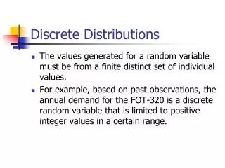
Further Illustration of Random Variables • A random variable corresponds to a quantitative interpretation of the outcomes of an experiment. • For example, a company offers its employees a drawing in its yearend party. A computer will randomly select an employee for the first prize of $100,000 based on the employees’ ID number, which ranges from 1 to 100.
In addition, the computer will randomly select two more employees for the second and third prizes of $50,000 and $10,000, respectively. • Assume that each employee can receive only one award and the drawing starts with the third prize and ends with the first prize. • Then, there are totally 100 × 99 × 98 = 970200 possible outcomes.
To Edward, whose employee ID number is 10, the random variable of his interest is as follows: X(<10, *, *>) = 10,000 X(<*, 10, *>) = 50,000 X(<*, *, 10>) = 100,000 X(all other outcomes) = 0 • To Grace, whose employee ID number is 30, the random variable of her interest is as follows: Y(<30, *, *>) = 10,000 Y(<*, 30, *>) = 50,000 Y(<*, *, 30>) = 100,000 Y(all other outcomes) = 0
The outcome spaces of random variables X and Y are identical. However, X and Y map some outcomes to different real numbers. • The spaces of X and Y are also identical and both are {0, 10000, 50000, 100000}. • The probability functions of X and Y are also equal. Prob(X=10,000) = Prob(Y=10,000) = 0.01 Prob(X=50,000) = Prob(Y=50,000) = 0.01 Prob(X=100,000) = Prob(Y=100,000) = 0.01 Prob(X=0) = Prob(Y=0) = 0.97
The expected values of X and Y are equal to E[X] = E[Y] = 10,000 * 0.01 + 50,000 * 0.01 + 100,000 * 0.01 = 1600.
Discrete Random Variables • Given a random variable X, let S denote the space of X. • If S is a finite or countable infinite set, then X is said to be a discrete random variable.
Countable Infinite • A set is said to be countable infinite, if it contains infinite number of elements and there exists a one-to-one mapping between each element of the set and the positive integers.
Examples of Countable / Uncountable Infinite • The set of integer numbers is countable. • The set of fractional numbers is countable. • The set of real numbers is uncountable.
Probability Mass Function • The probability mass function (p.m.f.) of a discrete random variable X is defined to be
In fact,the p.m.f. of a random variable is defined on a set of events of the experiment conducted. • In the previous drawing example, the set of outcomes that are mapped to 10,000 by X is an event.
Furthermore, in the previous drawing example, random variables X and Y map some outcomes to different real numbers. However, X and Y have the same distribution, i.e. the p.m.f. of X and the p.m.f. of Y are equal. More precisely,
Properties of the Probability Mass Function • The p.m.f. of a random variable X satisfies the following three properties:
Probability Distribution Function • For a random variable X, we define its probability distribution function F as
Properties of a Probability Distribution Function • Any function that satisfies these conditions above can be a distribution function.
An Example of the Probability Distribution Function of a Discrete Random Variable • Assume that we toss a 4-sided die twice. Then, we have 16 possible outcomes:
Operations of Random Variables • Let X and Y be two random variables defined on the same outcome space of an experiment. • Then, we can define a new random variable Z=f(X,Y).
For example, in the example of drawing, if Edward and Grace are husband and wife, then we can define a new random variable Z=X+Y. • We have X(<30, 10, *>) = 50,000 Y(<30, 10, *>) = 10,000 Z(<30, 10, *>) = 60,000
Function of Random Variables • Let X be a random variable and G be a function. Then, random variable Y=G(X)maps an outcome ν in the outcome space of X to value G(X(ν)). • With respect to the probability distribution functions, if G(X)is monotonically increasing, one-to-one mapping, then
An Example of Functions of Random Variables • Let random variable X be the sum of two tosses of a 4-sided die and Y=X2. • Then,
Expected Value of a Discrete Random Variable • Let X be a discrete random variable and S be its space. Then, the expected value of X is • μ is a widely used symbol for expected value.
Expected Value of a Function of a Random Variable • Let X be a random variable and G be a function. Then, the expected value of random variable is equal to
For example, let X correspond to the outcome of tossing a die once. Then, Px(1)=Px(2)=Px(3)=Px(4)=Px(5)=Px(6)=1/6. and E[X]=3.5 • If we are concerned about the difference between the observed outcome and the mean. And define Y=|X-E[X]|, then PY(1/2)=1/3, PY(3/2)=1/3, PY(5/2)=1/3.
Theorems about the Expected Value (a)If c is a constant, (b)If c is a constant and g is a function, (c)If c1 and c2 are constants and g1 and g2 are functions, then
Theorems about the Expected Value • Proof of (a): Trivial. • Proof of (b):
Theorems about the Expected Value • Proof of (c): • An extension of (c)
Variance of a Discrete Random Variable • The variance of a random variable is defined to be and is typically denoted by σ2. • For a discrete random variable X, • σ is normally called the standard deviation.
Variance of a Discrete Random Variable • Let X be a random variable with mean μX and variance σX2. Let Y= aX+b, where a and b are constants. Then,
Variance of a Random Variable • The variance of a random variable measures the deviation of its distribution from the mean. • For example, in one drawing, Robert has 0.1% of chance to win $100,000, while in another drawing, he has 0.01% of chance to win $1,000,000.
The expected amounts of award in these two drawings are equal. 0.001 * 100000 = 100 0.0001 * 1000000 = 100 • However, their variances are different. 0.001 * (100000 – 100)2 + 0.999 * (0 – 100)2 = 9,990,000 0.0001 * (1000000 – 100)2 + 0.999 * (0 – 100)2 = 99,990,000
In many distributions, the mean and variance together uniquely determine the parameters of the random variables.
The Bernoulli Experiment and Distribution • A Bernoulli experiment is a random experiment, the outcome of which can be classified in one of two mutually exclusive and exhaustive ways, say, success and failure. • A sequence of Bernoulli trials occurs when a Bernoulli experiment is performed several independent times, so that the probability of success, say p, remains the same from trial to trial.
The Bernoulli Distribution • Let X be a Bernoulli random variable. The p.m.f of X can be written as where k= 0 or 1 and p is the probability of success. • The expected value of X is • The variance of X is
The Binomial Distribution • Let X be the random variable corresponding to the number of successes in a sequence of Bernoulli trials. • Then, where n is the number of Bernoulli trials and p is the probability of success in one trial. • X is said to have a binomial distribution and is normally denoted by b(n , p).
Example of the Binomial Distribution • Assume that Tiger and Whale are the two teams that enter the Championship series of the professional basket ball league. Based on prior records, Tiger has a 60% chance of beating Whale in a single game. Larry, who is a fan of Tiger, makes a bet with Peter, who is a fan of Whale. According to their agreement, Larry will pay Peter $1000, should Whale win the 5-game series. In order to make a fair bet, how much should Peter pay Larry, if Tiger wins the series?
If the championship series consists of 3 games, then what is the probability that Tiger win the series?
The Moment-Generating Function • Let X be a discrete random variable with p.m.f and space S. If there is a positive number h such that exists and is finite for -h<t<h, then the function of t defined by is called the moment-generating function of X. and often abbreviated as m.g.f.
The Moment-Generating Function • Let X and Y be two discrete random variables with the same space S. If then the probability mass functions of X and Y are equal. • Insight of the argument above: Assume that S={s1,s2, …, sk}contains only positive integers. Then, we have Therefore, , i.e. X and Y have the same p.m.f.
The Moment-Generating Function • Let be the m.g.f of a discrete random variable X. Furthermore, • In particular,
The Moment-Generating Function of the Binomial Distribution • Let X be b(n , p). are both difficult to compute.
On the other hand, we can easily derive the m.g.f. of a binomial distribution.
The Moment-Generating Function of the Binomial Distribution Therefore,