Time Series Forecasting Tool: Techniques and Applications
220 likes | 279 Vues
Explore the importance of demand forecasting, methods of time series forecasting, and applications for business decision-making. Understand the significance of data analysis in predicting future trends and optimizing supply chain efficiency.

Time Series Forecasting Tool: Techniques and Applications
E N D
Presentation Transcript
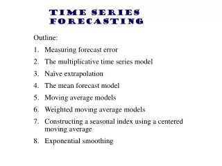
Text: Chapter 13 Time Series Forecasting Toolse.g. Moving Average, Exponential Smoothing
Motivation: Demand Forecast • Think of a Business Plan, product or service you provide • Discussion: • Why is there a need to forecast future demand? • How would you forecast future demand? • Does the type & availability of information / data matter? • e.g. past sales data • “Forward” sales intelligence e.g. market research ; Buyers’ intentions • Novel product / service: Gut feeling? ; Experts’ opinions? • Does forecast horizon matter i.e. short, medium, long term? • Case Studies • Kmart / Manufacturers uses Weather Forecasts to plan inventory stock • HP uses regression model to forecast demand for printers
Evidence indicates: A “good” demand forecast • Defines the success of the Supply Chain • Operational Efficiency: Sourcing, staffing, capital investment, logistics, … • Is a Collaborative process internally & externally • Internally: R & D, Marketing, Finance etc. forecast “together” • Externally: Forecasts from agents ; feedback from customers etc. • i.e. concensus-driven and a shared ownership ; needs regular update • Defined by its degree of usefulness / adoption rather than accuracy (“6 Rules for Effective Forecasting” HBR Jul-Aug 2007)
Forecasting Methods Empirical Evidence: No one method is superior. Hybrid method (quantitative+qualitative) enhances accuracy / mitigates bias e.g. HBR Article “6 Rules for Effective Forecasting”
Analytical Forecasting Tools • Regression Forecasting: • Demand = f(Price, Competitor’s Price, Business Cycle, Life Cycle, …) • Profit = f(time) e.g. uniform or straight line relationship over time • Time Series Forecasting: Extrapolation of past patterns • Non-uniform relationship over time
Business & Product Life cycles Demand Business Cycle Recession Product Life Cycle e.g. Cellular Phones Inflation 2G Recovery 3G Depression 1G time time
Quantitative Forecasting Methods Note: Regression Method “explains” demand Time Series Methods extrapolate past data patterns
Statistically Speaking • Time Series : Collection of data recorded over time • Daily #Breakdowns; Monthly downtimes ; Quarterly Productivity ; Annual Profit. • Data variability : Data is dynamic i.e. fluctuate with time • Forecast : Prediction of future using current & past data • Backcast: What should “present” be given “future” ? • Eg. Intakes of personnel / Engineering/ Science students determined by backcasting specified future R&D personnel. • Backcasting = Forecasting on “reverse” time scale.
Coverage • Regression Models using Time as a predictor • Time Series Forecasting Tools • Naïve Forecast (i.e. Random Walk): • Forecast of next lag,F(t+1)=Current Data, Y(t) • Moving Average: • F(t+1) = Average [Y(t), Y(t-1), Y(t-2),…] eg Avg(Today, Yesterday, …] • Exponential Smoothing: • For data w/o trend F(t+1) = Weighted Average [Y(t), Y(t-1), Y(t-2),…] • For data with Trend : Holt Method • For data with Trend & Seasonality : Winters Method • Benchmarking / Monitoring Forecasting Accuracy • Forecast error metrics: MAD ; MSE ; MAPE • Monitoring Forecasting Quality: Tracking Signal
Trend Models • P-order model:Data is a function of time • Autoregressive model:Data is a function of its past * * * * Parsimony: Select low-order p * * * * * * * *
Growth Models • Constant Growth Model: e.g. Moore’s Law: Computer chip “power” doubles every 18 months Applications (1) Monthly growth in Singapore’s Foreign Reserves (2) Microsoft Profit CAGR (3) China’s annual forex reserves growth • Product Life Cycle Model • Requires (subjective) input on Saturation Level S, Time of maximum growth I and degree of initial pent-up demand F • Initial data helpful in estimating I & F. t
New Product Forecasting: A Life-Cycle Model i.e. S-Curve Saturation Level, S (eg market research) Discuss: How is S-curve Connected to Bell Curve? Half Life: Demand = ½ S Demand Delay Factor, F Inflection Point, I Time, t
Simplest Time Series Tool:Naïve Forecasting Y(t) if no trend Y(t) + [Y(t)-Y(t-1)], if trend present F(t+1) Y(t), Current Data t Applicability:Very short (eg 1 lag ahead) for stable process Examples:Machine / Personnel Assignment ; Stock Market ; Quality Control ; Maintenance Planning
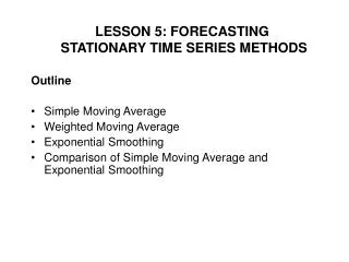
Time Series Forecasting via Smoothing Methods • Data smoothing = Data “massaging” Averaging “zeroes out” variability to reveal trend. • Two smoothing techniques: • Moving Average • Exponential Smoothing
Moving Average • Average of moving window of data eg 3 period MA: Forecast F(t+1)= [Y(t-2) + Y(t-1) + Y(t)] / 3 • Shortcomings • Window length: Why not MA(4), MA(5) etc. • Valid for flat / non-trending TS • Why use equal weights in averaging past data ? v/s say F(t+1) = 0.2 Y(t-2) + 0.3 Y(t-1) + 0.5 Y(t) • Application: Demand Intensity for COE 1 2 3 F(4) 2 3 4 F(5) 3 4 5 F(6)
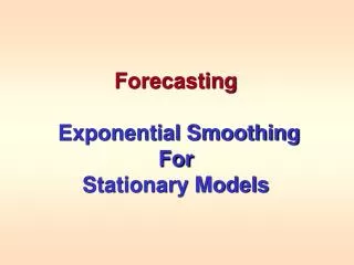
L(t-1) F(t+1) Y(t) Simple Exponential Smoothing for “NON-TRENDING” Time Series • Define L(t-1)= WeightedAvg of Y1, Y2, …,Y(t-1) • => L(t) = Weighted Average of Y(t) and L(t-1) = a Y(t) + (1-a) L(t-1), = Forecast (t+1) • a = 1 => Naïve Forecast ; a = 0 => Y(t) “not credible” & ignored by forecast • Start with F(2) = L(1) = Y(1) • F(3) = L(2) = a Y(2) + (1-a) Y(1) • F(4) = L(3) = • Concept:Forecast = exponentially weighted average of Present & Past! • Problem: Which exponential weight a to use? • Case Study: Demand Intensity for COE Exponential Weights .7 .21 .09
Benchmarking Forecasting Accuracy • Good Forecasts small forecasting errors. • 3 commonly-used benchmarks: • Mean Absolute Deviation, MAD = • Mean Squared Error, MSE = • Mean Absolute Percentage Error, MAPE = • Minimize (any) forecasting error metrics above to obtain “optimal” forecasting model
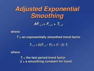
Holt Smoothing for Trending TS • Generalization of simple exponential smoothing • Updates Level and Trend i.e. weighted average of PRESENT and PAST • = weighted average of • = weighted average of slopes • Applications: COE$ & Australian Wine Grape Production
Winters Exponential Smoothing Model for Trend & Seasonality • Generalization of simple exponential smoothing • Updates (deseasonalized) level, trend and seasonality components • Produces “seasonal” forecast • Applications: Singapore GDP S = 1 =>Holt Winters
Seasonal Indices: Application • Application: Calendar Sales Plan for Major Oil Company Country Yearly Sales Target = 838 mbbl • Target: Better Delivery Planning using Seasonal Indices Jan Feb Mar Apr May Jun Jul Aug Sep …. Actual Sales 57 45 73 72 71 73 63 62 78 …. Delivery Plan 70 70 70 70 70 70 70 70 70 …. % Sales / Plan 81 64 104 103 101 104 90 89 112 …. Calendar Plan 63 46 74 78 75 70 63 61 76 …. (= 70 x monthly seasonal index) % Sales / CP 90 98 99 92 95 104 100102 103
Hallmarks of Good Forecasting • Forecasting Horizon • Long: Expert ; Medium: Regression ; Short: Time Series Methods • Inspect time series • “Constant Level”: Moving Average / Simple Exponential Smoothing • Trends & Seasons: Holt / Winters ES • Forecasts should be • Based on good-quality data o/w GIGO (Garbage-in-garbage-out) • Timely to allow planning • Monitored for reliability / quality (see next slide) • Simple and easy to obtain via software e.g. MS Excel, SPSS, Forecast Pro (http:://www.ForecastPro.com) etc.
Parting Thoughts • More complicated Time Series methods: ARIMA, State Space,.. • Emerging Forecasting Tool: Neural Networks • Uses Artificial Intelligence (mimics human reasoning) to detect patterns in data ; “Black box” Complexity • Long Term Asset Management ($b debacle !) was a user! • Another forecasting model for new technology / product: Bass Model • Based on Diffusion of Innovations i.e. 2.5% innovators, 13.5% early adopters, … • Business Success begins with a Good Forecast!