Weather Charts Analysis: Geostrophic and Thermal Wind Patterns
50 likes | 148 Vues
Analysis of geostrophic and thermal wind patterns on weather charts from July 3, 2006, at 300mb and 700mb levels. Calculations and comparisons of wind speeds, geopotential gradients, and thermal wind effects. Interpretation of temperature differentials and surface front implications.

Weather Charts Analysis: Geostrophic and Thermal Wind Patterns
E N D
Presentation Transcript
Weather charts, 3 July 2006 300 mb • Consider the geopotential gradient across the solid red line. • Δz = 952 – 912 Dm = 400 m, ΔΦ = 4000 m2 s-2 • Δx = 5.5 deg lat = 616 km (1 deg = 111 km) • pΦ = 4000 / 616000 = 0.0065 m s-2 • Ug = f-1 k x pΦ = 54 ms-1 (f = 1.12 x10⁻⁴) • Ug = 105 kt compared with 100-105 kt measured (1 knot = I nautical mile hr-1= 1852 m hr-1 = 0.514 ms-1)
700 mb • Consider the geopotential gradient across the solid red line. • Δz = 316 – 300 Dm = 160 m, ΔΦ = 1600 m2 s-2 • Δx = 5.5 deg lat = 616 km (1 deg = 111 km) • pΦ = 1600 / 616000 = 0.0026 m s-2 • Ug = f-1 k x pΦ = 23 ms-1 (f = 1.12 x10⁻⁴) • Ug = 45 kt compared with 45 kt measured (1 knot = I nautical mile hr-1= 1852 m hr-1 = 0.514 ms-1)
Thermal wind 700 mb 300 mb Camborne temperature at 700 mb = 5°, at 300 mb = -37° Valentia temperature at 700 mb = -1°, at 300 mb = -40° ΔT = 6° at 700 mb, 3° at 300 mb, mean around 4.5° Δx = 3.7 degrees latitude = 411 km T = 1.13x10⁻⁵ K m-1 ΔUg = - (r/f) T Δln p = (286x104) 1.13x10⁻⁵ ln(7/3) = 27 ms-1 Actual value is 30 ms-1 but the calculation is considerably cruder than the 3-figure precision implies.
Surface chart Temperature gradient coincides with a front