Download

1 / 32
320 likes | 468 Vues
Force Panel IDENTIFICATION OF HUMAN TRANSFER FUNCTION. 2. Human Transfer Function. H( w ). Reference position (to be followed by the finger). Actual finger position. 3. Modelling. The considered HTF to find are:. 1). 2). 3). Class work Identification in frequency.

E N D
Force Panel IDENTIFICATION OF HUMAN TRANSFER FUNCTION
2 Human Transfer Function
H(w) Reference position (to be followed by the finger) Actual finger position 3 Modelling
The considered HTF to find are: 1) 2) 3)
Class work Identification in frequency
1th work in class: filter outliers due to low finger pressure Main steps – 1 filter outliers
Show and run the file “PROPEDEUTICO_Filtra Outliers.m” Main steps – 1.a Filter outliers with heuristics
Possible ideas to identify outliers: • Identify them with an upper value [use ‘find’] • identify them with the derivative [use ‘diff’] • To replace the outliers values: • With the previous value • with the mean value between the previous and the following • interpolating • After outliers compensation compare the FFT of the original and the filtered signal [use ‘fft’] Main steps – 1.a Filter outliers with heuristics
A stationary signal x(t)=cos(2*pi*10*t)+cos(2*pi*25*t)+cos(2*pi*50*t)+cos(2*pi*100*t) http://users.rowan.edu/~polikar/WAVELETS/WTpart1.html Main steps – 1.b Filter outliers with Wavelets
Why wavelets? They are extremely useful in non-stationary signals a signal with four different frequency components at four different time intervals, hence a non-stationary signal. The interval 0 to 300 ms has a 100 Hz sinusoid, the interval 300 to 600 ms has a 50 Hz sinusoid, the interval 600 to 800 ms has a 25 Hz sinusoid, and finally the interval 800 to 1000 ms has a 10 Hz sinusoid. Main steps – 1.b Filter outliers with Wavelets
Why wavelets? They are extremely useful in non-stationary signals Main steps – 1.b Filter outliers with Wavelets
How can appear a wavelet: the Morlet wavelet shown is defined as the product of a complex exponential wave and a Gaussian envelope: http://paos.colorado.edu/research/wavelets/wavelet2.html Main steps – 1.b Filter outliers with Wavelets
we now need some way to change the overall size as well as slide the entire wavelet along in time. We thus define the "scaled wavelets" as: We are given a time series X, with values of xn, at time index n. Each value is separated in time by a constant time interval dt. The wavelet transform Wn(s) is just the inner product (or convolution) of the wavelet function with our original timeseries: W(s, n) Main steps – 1.b Filter outliers with Wavelets
The above integral can be evaluated for various values of the scale s (usually taken to be multiples of the lowest possible frequency), as well as all values of n between the start and end dates. A two-dimensional picture of the variability can then be constructed by plotting the wavelet amplitude and phase. scale Main steps – 1.b Filter outliers with Wavelets
The wavelets allow to decompose a signal as follows: the DWT (Discrete Wavelet Transform) The DWT analyzes the signal at different frequency bands with different resolutions by decomposing the signal into a coarse approximation and detail information. DWT employs two sets of functions, called scaling functions and wavelet functions, which are associated with low pass and highpass filters, respectively. The decomposition of the signal into different frequency bands is simply obtained by successive highpass and lowpass filtering of the time domain signal. The original signal x[n] is first passed through a halfband highpass filter g[n] and a lowpass filter h[n]. After the filtering, half of the samples can be eliminated according to the Nyquist's rule, since the signal now has a highest frequency of p /2 radians instead of p . The signal can therefore be subsampled by 2, simply by discarding every other sample. Main steps – 1.b Filter outliers with Wavelets
This constitutes one level of decomposition and can mathematically be expressed as follows: (where yhigh[k] and ylow[k] are the outputs of the highpass and lowpass filters, respectively, after subsampling by 2) Main steps – 1.b Filter outliers with Wavelets
The above procedure, which is also known as the subband coding, can be repeated for further decomposition. At every level, the filtering and subsampling will result in half the number of samples (and hence half the time resolution) and half the frequency band spanned (and hence double the frequency resolution). Detail of level 1 Detail of level 2 Detail of level 3 Approximation of level 3 Main steps – 1.b Filter outliers with Wavelets
One important property of the discrete wavelet transform is the relationship between the impulse responses of the highpass and lowpass filters. The highpass and lowpass filters are not independent of each other, and they are related by where g[n] is the highpass, h[n] is the lowpass filter, and L is the filter length (in number of points). Note that the two filters are odd index alternated reversed versions of each other. Lowpass to highpass conversion is provided by the (-1)n term. Filters satisfying this condition are commonly used in signal processing, and they are known as the Quadrature Mirror Filters (QMF). Main steps – 1.b Filter outliers with Wavelets
a quadrature mirror filter is a filter whose magnitude response is mirror image about p/2of that of another filter. Together these filters are known as the Quadrature Mirror Filter pair. The filter responses are symmetric about : The analysis filters are often related by the following formulae in addition to quadrate mirror property: In this way they are also complemetary and there fore the signal is not distorted!!! Main steps – 1.b Filter outliers with Wavelets
Show an example with wavemenu Main steps – 1.b Filter outliers with Wavelets
2th work in class: filter the frequency ratio (that is too noisy to be used as it is) zoom Zoom of the zoom Main steps – 2 filter the FFT ratio
3th work in class: fit the modulus Main steps – 3 fit the modulus of the HTF
4th work in class: find the phase Main steps – 4 find the HTF delay (t)
% program to complete in class % [to do between square brackets] % so, find '[]' to localize where to write code (or functions) clear all close all; clc; %% Load DATA % [1.] % [copy the filename to elaborate and its directory] im = strcat('Dati/Segnale_5/fp_acq_03_04_20111004115703.txt'); [header, hh, dd] = readColData(im,8,7,1); tempo = dd(:,1); % time x = dd(:,2); % x finger position red by arduino [ bit ] y = dd(:,3); % y finger position red by arduino [ bit ] f1 = dd(:,4); % first load cell red by arduino [ bit ] f2 = dd(:,5); % second load cell red by arduino [ bit ] f3 = dd(:,6); % third load cell red by arduino [ bit ] x_segnale = dd(:,7); % x reference of the vertical line [ pixel ] x_touch = x * 1.19 - 108.55 ; % x finger position with respect to LCD (calibration) [ pixel ] ID = dd (:, 8 ) ; Class work
% extract time tempo = tempo - tempo(1) ; Tc = tempo(end) / length(tempo) ; tempo = 0 : (length(tempo) - 1) ; tempo = tempo * Tc ; % filter repeated data on the ARDUINO ID IIf = find( [ 1; diff(ID)] ) ; data_finger = x_touch( IIf ) ; % x finger position filtered data_input = x_segnale( IIf ) ; % x reference filtered tempo = tempo( IIf ) ; % time filtered tempo = tempo - tempo(1) ; figure, plot( tempo/1000, data_finger, 'b', tempo/1000, data_input, 'r' ) title('Reference and finger position'), grid on %% 1. Filtering outliers % [filtrare i salti dovuti a scarsa pressione del dito] meanF = mean (f1(IIf) + f2(IIf) + f3(IIf)) ; % mean of the load figure, plot( tempo/1000, data_finger, 'b', tempo/1000, (f1(IIf) + f2(IIf) + f3(IIf) - meanF) *10 + 300, 'r' ) title('Finger position and applied force'), grid on % [1.] soglia_Dx = 100 ; data_finger = FiltraOutliers_CELLE(data_finger, data_input, soglia_Dx) ; Class work
%% 2. Trasfer Function estimation data_input = data_input - mean(data_input) ; data_finger = data_finger - mean(data_finger) ; % FFT computation F_Iinput = fft(data_input) / length(data_input) ; F_Ooutput = fft(data_finger) / length(data_finger) ; % plot of the transform ratio Hs = F_Ooutput ./ F_Iinput ; Hs(1) = 1 ; % (to recover the fact that the mean values were just eliminated) ffTF = 1000 * ( 0:(length(data_input)-1) ) / tempo(end) ; % Frequency vector [Hz] figure, plot(ffTF, abs(F_Iinput), 'r'), hold on plot(ffTF, abs(F_Ooutput)) plot(ffTF, abs(Hs), 'c') legend('Input','Output','Hs') xlabel ('Frequency [Hz]') % [] % [to filter the experimental transfer function 'Hs' just obtained by FFT ratio] plotta = 1 ; Hs = Filtro_Hs( Hs, F_Iinput, F_Ooutput, ffTF, plotta ) ; Class work
%% just rename the variables: Iinput = data_input ; Ooutput = data_finger ; %% 3. FITTING modulus with lsqnonlin % [] % write a function 'FittingFrequenza' % par_ini = [0 2*pi*0.2 2*pi*0.1 2*pi*2] % solo primo ordine, 4 par par_ini = [0 2*pi*0.2 2*pi*0.1 0.7 2*pi*2] % anche secondo ordine, 5 par if length(par_ini) == 4 % 1th order par_ott = lsqnonlin(@(par) FittingFrequenza(par, Hs, ffTF, 0), par_ini, ... [0 0 0 0], [100 100 100 100]) ; elseif length(par_ini) == 5 % 2nd order par_ott = lsqnonlin(@(par) FittingFrequenza(par, Hs, ffTF, 0), par_ini, ... [0 0 0 0 0], [100 100 100 100 100]) ; % con [0 100 90 0 0] si fa 2d ordine end Class work
%__________________________________ % % 4. estimate the parameter delay %__________________________________ % [] % write a function simulink 'CompDinamica' that simulates the model without delay % use the function 'corr' to estimate the delay % 0. neglect the mean values Iinput = Iinput - mean(Iinput) ; Ooutput = Ooutput - mean(Ooutput) ; % 1. dynamical simulation without delay par = par_ott ; if length(par) == 4 % solo primi ordini sim('CompDinamica_1ord') elseif length(par) == 5 % secondo ordine sottosmorzato sim('CompDinamica_2ord') end Comp_Iinput = interp1(time, Comp_Iinput, tempo/1000)' ; Class work
% 2. correlation of the output with the simulated output (without delay) % [] % [use the function 'corr'] tau = 0 ; par_ott(1) = tau ; % plot results FittingFrequenza(par_ott, Hs, ffTF, 1) ; % !!!!!!!!!!!!!!!!!!!!!!!!! ModelloHTF(par_ott, ffTF, 1) ; %% SIMULATION OF A STEP INPUT WITH THE HTF par = par_ott ; if length(par) == 4 % 1th order sim('simulazione_1ord') elseif length(par) == 5 % 2nd order sim('simulazione_2ord') end figure, plot(time, step, time, step_out), title('Step input simulation') Class work