Properties of Filter (Transfer Function)
Properties of Filter (Transfer Function). Real part of a Transfer Function for different order periodic filters. . Transfer Function Variation At Different Nodes for the Sixth Order Non-Periodic Filter. Real part. T.F . (Real). Transfer function overshoot for near boundary nodes.

Properties of Filter (Transfer Function)
E N D
Presentation Transcript
Properties of Filter (Transfer Function) Real part of a Transfer Function for different order periodic filters.
Transfer Function Variation At Different Nodes for the Sixth Order Non-Periodic Filter Real part T.F. (Real) Transfer function overshoot for near boundary nodes Numerical instability at nodes 2 and 3 Imaginary part T.F. ( Imaginary) Excessive dissipation at nodes N-1 and N-2 Imaginary parts affect dispersion properties
Real partof the Transfer Function for the Composite Filter ** At nodes 2 and N-1 : Second order filter stencil 3 and N-2 : Fourth order filter stencil 4 to N-3 : Sixth order filter stencil ** LOC approach – Chu & Fan (JCP 1998) , Gaitonde & Visbal (AIAA 2000)
Numerical StabilizationProperty of the Filters Initial condition Kh = 0.2π Nc = 0.1 C = 0.1 Solution at t =30 Solution of 1D wave equation by unconditionally unstable CD2 spatial discretization and Euler time discretization. Application of the given filter stabilize the solution.
Comparison ofNumerical Amplification Factor Contours, With and Without Applying Filter Without Filter , 6th Order Filter Scaled numerical amplification contours for the solution of 1D wave equation, when the spatial discretization is carried out by OUCS3 and time discretization is obtained by RK4.
Numerical Stabilization Property of the Filters Recommended central filters: 1) 4th order filter with value very close to 0.5 2) 2nd order filter apply infrequently
Effect of Frequency of Filtering on the Computed Solution n: Filtering interval This procedure can be used for any order filter in any directions.
Effect of Direction of Filtering on the Computed Solution • Azimuthal filters smears • vorticity in that direction and are not preferred over the full • domain. Although, it is acceptable near the boundary. • In the rest of the domain, use radial filters (could be central or upwinded variety).
Filtered solution 6th order azimuthal filter for 30 lines, = 0.49 6th order radial filter for complete domain , = 0.45 Re = 150, A =2 ,ff/f0 = 1.5 Experimental flow visualization picture (Thiria et. al. (2006)) Unfiltered solution
Transfer Function Variation At Different Nodes for the Given Filter Coefficients T.F. (Real) Real Part T.F. (Imaginary) Imaginary Part
Comparison ofReal Part of Transfer Function, for Different Upwind Coefficients T.F. (Real) T.F. (Real) Transfer functions are plotted for interior nodes only.
Comparison ofImaginary Part of Transfer Function, for Different Upwind Coefficients T.F. (Imaginary) T.F. (Imaginary) Transfer functions are plotted for interior nodes only.
Benefits of upwind filter • Problems of higher order central filters have been diagnosed as due to numerical instability near the boundary and excessive dissipation. These can be rectified by the upwind filter. • The upwind filter allows one to add controlled amount of dissipation in the interior of the domain. Absolute control over the imaginary part of the TF allows one to mimic the hyper-viscosity / SGS model used for LES.
Comparison ofNumerical Amplification Factor Contours,for Different Upwind Coefficients Scaled numerical amplification contours for the solution of 1D wave equation, when the spatial discretization is carried out by OUCS3 and time discretization is obtained by RK4.
Comparison of ScaledNumerical Group Velocity Contours,With and Without Upwind Filter Scaled numerical group velocity contours for the solution of 1D wave equation, when the spatial discretization is carried out by OUCS3 and time discretization is obtained by RK4.
Filtered solution 6th order azimuthal filter for 30 lines, = 0.49 6th order radial filter for complete domain , = 0.45 η = 0.001 Re = 150, A =2 ,ff/f0 = 1.5 Experimental flow visualization picture (Thiria et. al. (2006)) Unfiltered solution
Comparison of Flow Field Past NACA-0015 Airfoil t = 1.92 Flow Direction Experimental visualization 8th order azimuthal filter 6th order azimuthal filter = 0.48 = 0.48 6th order azimuthal filter for 30 lines, 6th order azimuthal filter for 60 lines, = 0.485 = 0.485 5th order upwind wall-normal filter, η = 0.001 5th order upwind wall-normal filter, η = 0.001
Comparison of Flow Field Past NACA-0015 Airfoil t = 2.42 Flow Direction Experimental visualization 8th order azimuthal filter 6th order azimuthal filter = 0.48 = 0.48 6th order azimuthal filter for 30 lines, 6th order azimuthal filter for 60 lines, = 0.485 = 0.485 5th order upwind wall-normal filter, η = 0.001 5th order upwind wall-normal filter, η = 0.001
Recommended Filtering Strategy • Optimal filter is a combination of azimuthal central filter applied close to the wall with a non-periodic fifth order upwinded filter for the full domain. • This has similarity with DES (Barone & Roy (2006), Nishino et. al (2008) and Tucker (2003)), but does not require solving different equations for different parts of the domain. • One does not require turbulence or SGS models. • Hence this process is also computationally efficient in terms of computational efforts and cost.
Conclusions 1) Non-periodic filters cause numerical instability near inflow and excessive damping near outflow. 2) This problem can be removed by using a new upwind composite filter which even allows one to add controlled amount of dissipation in the interior of the domain. 3) Upwind filter has a better dispersion properties as compared to conventional symmetric filters. 4) This approach of using upwind filter does not require using different equations in the different parts of the domain. Also one does not need any turbulence or SGS models resulting in a fewer and faster computations.
THANK YOU Look for us at: http://spectral.iitk.ac.in