
SlideServe
Menu
Préférences
© SlideServe · v2026

Loop Transfer Function

lois avatar
19 diapositives · 604 Views · Jul 27, 2014

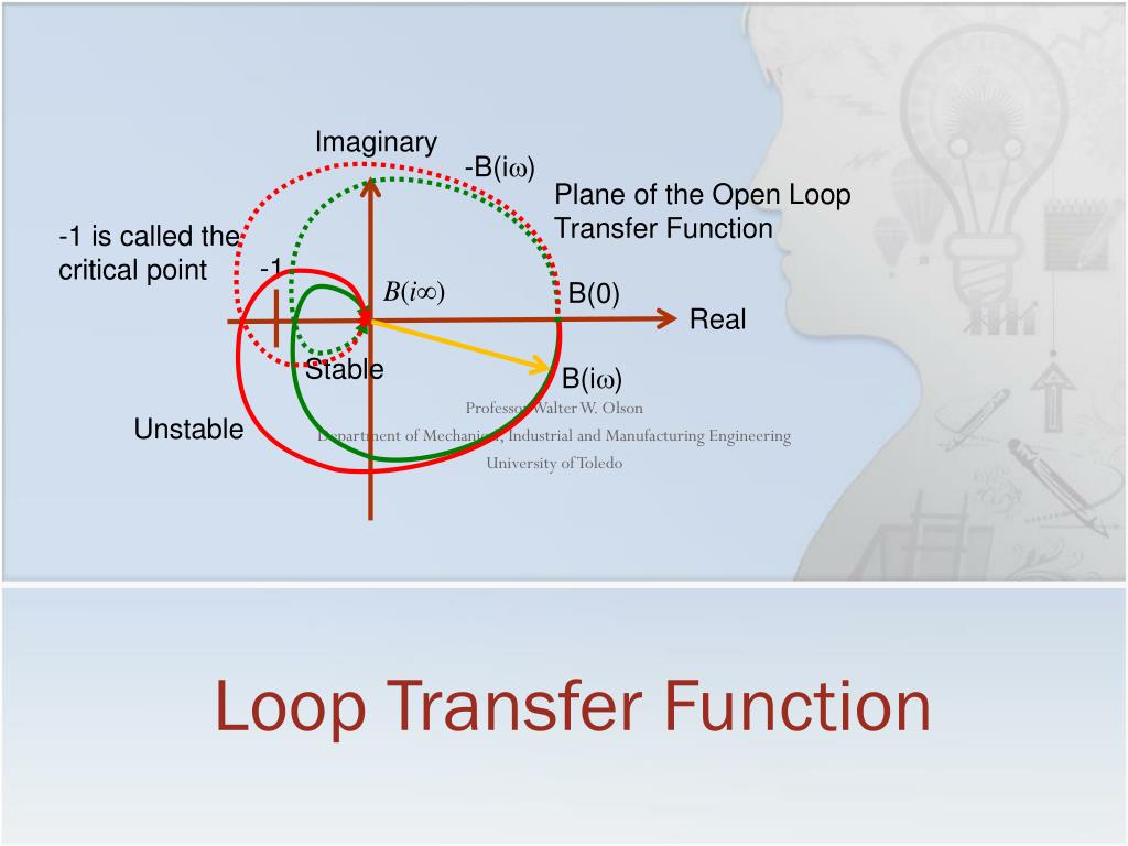
Loop Transfer Function. Imaginary. -B( i w ). Plane of the Open Loop Transfer Function . -1 is called the critical point. -1. B(0). Professor Walter W. Olson Department of Mechanical, Industrial and Manufacturing Engineering University of Toledo. Real. Stable. B( i w ). Unstable.
Loop Transfer Function - slide 1
01 / 19Loop Transfer Function
1 / 17

Télécharger la présentation

Loop Transfer Function
Une image / un lien ci-dessous est fourni (tel quel) pour télécharger la présentation

Politique de téléchargement : le contenu du site vous est fourni TEL QUEL pour votre information et votre usage personnel ; il ne peut être vendu, concédé sous licence ni partagé sur d’autres sites sans l’accord de son auteur.Le contenu vous est fourni TEL QUEL, pour votre information et votre usage personnel uniquement. Téléchargez la présentation en cliquant sur ce lien. Lors du téléchargement, si vous ne parvenez pas à télécharger une présentation, l’éditeur a peut-être supprimé le fichier de son serveur.Pendant le téléchargement, si vous ne parvenez pas à obtenir une présentation, le fichier a peut-être été supprimé par l’éditeur.

F I N

Plus de contenu associé

Transcription de la présentation
  1. Loop Transfer Function Imaginary -B(iw) Plane of the Open Loop Transfer Function -1 is called the critical point -1 B(0) Professor Walter W. Olson Department of Mechanical, Industrial and Manufacturing Engineering University of Toledo Real Stable B(iw) Unstable

  2. Outline of Today’s Lecture • Review • Partial Fraction Expansion • real distinct roots • repeated roots • complex conjugate roots • Open Loop System • Nyquist Plot • Simple Nyquist Theorem • Nyquist Gain Scaling • Conditional Stability • Full Nyquist Theorem

  3. Partial Fraction Expansion • When using Partial Fraction Expansion, our objective is to turn the Transfer Functioninto a sum of fractions where the denominators are the factors of the denominator of the Transfer Function:Then we use the linear property of Laplace Transforms and the relatively easy form to make the Inverse Transform.

  4. Case 1: Real and Distinct Roots

  5. Case 1: Real and Distinct RootsExample

  6. Case 2: Complex Conjugate Roots

  7. Case 3: Repeated Roots

  8. Heaviside Expansion

  9. Loop Nomenclature Disturbance/Noise Reference Input R(s) Error signal E(s) Output y(s) Controller C(s) Plant G(s) Prefilter F(s) Open Loop Signal B(s) Sensor H(s) + + - - The plant is that which is to be controlled with transfer function G(s) The prefilter and the controller define the control laws of the system. The open loop signal is the signal that results from the actions of the prefilter, the controller, the plant and the sensor and has the transfer function F(s)C(s)G(s)H(s) The closed loop signal is the output of the system and has the transfer function

  10. Closed Loop System Error signal E(s) Output y(s) Input r(s) Controller C(s) Plant P(s) Open Loop Signal B(s) -1 + +

  11. Note: Your book uses L(s) rather than B(s) To avoid confusion with the Laplace transform, I will use B(s) Open Loop System Error signal E(s) Output y(s) Input r(s) Controller C(s) Plant P(s) Open Loop Signal B(s) Sensor -1 + +

  12. Open Loop SystemNyquist Plot Error signal E(s) Output y(s) Input r(s) Controller C(s) Plant P(s) Open Loop Signal B(s) Imaginary B(-iw) Plane of the Open Loop Transfer Function Sensor -1 -1 B(0) Real + + B(iw) -1 is called the critical point

  13. Simple Nyquist Theorem Error signal E(s) Output y(s) Input r(s) Imaginary Controller C(s) Plant P(s) -B(iw) Plane of the Open Loop Transfer Function Open Loop Signal B(s) -1 is called the critical point -1 B(0) Sensor -1 Real Stable B(iw) Unstable + + Simple Nyquist Theorem: For the loop transfer function, B(iw), if B(iw) has no poles in the right hand side, expect for simple poles on the imaginary axis, then the system is stable if there are no encirclements of the critical point -1.

  14. Example • Plot the Nyquist plot for Im -1 Re Stable

  15. Example • Plot the Nyquist plot for Im -1 Re Unstable

  16. Nyquist Gain Scaling • The form of the Nyquist plot is scaled by the system gain • Show with Sisotool

  17. Conditional Stabilty • While most system increase stability by decreasing gain, some can be stabilized by increasing gain • Show with Sisotool

  18. Full Nyquist Theorem • Assume that the transfer function B(iw) with P poles has been plotted as a Nyquist plot. Let N be the number of clockwise encirclements of -1 by B(iw) minus the counterclockwise encirclements of -1 by B(iw)Then the closed loop system has Z=N+P poles in the right half plane. • Show with Sisotool

  19. Summary • Open Loop System • Nyquist Plot • Simple Nyquist Theorem • Nyquist Gain Scaling • Conditional Stability • Full Nyquist Theorem Im -1 Re Unstable Next Class: Stability Margins