Download
1 / 22
220 likes | 336 Vues
A Method for Measuring the Photoionization of Neutral Gas by Soft X-Rays. Edward B. Jenkins Princeton University Observatory. Principal Issues. Relevance to the study of DLAs Monitor the strength and character of the soft X-ray environment that irradiates the gas from Internal sources

E N D
A Method for Measuring the Photoionization of Neutral Gas by Soft X-Rays Edward B. Jenkins Princeton University Observatory
Principal Issues • Relevance to the study of DLAs • Monitor the strength and character of the soft X-ray environment that irradiates the gas from • Internal sources • Radiation from embedded hot gas • Population of very hot stars emitting EUV radiation • The effects of an external penetrating radiation • Metagalactic flux • AGN radiation for proximate DLAs (PDLA). • Obtain an understanding of how measurements of element abundances could be influenced by this type of radiation that can penetrate H I regions.
Requirements for a Reliable Interpretation • Considerations for the choice of species to compare – should be immune to uncertainties arising from the following: • Overall metallicity level • The effects of element depletions caused by dust formation • [α/Fe] • [secondary elem./primary elem.] • Contributions from H II regions • There must be a workable selection of absorption lines.
An Ideal Combination:Neutral Argon and Oxygen • Basic premises: • Ar and O are both α-process elements. • They are not subject to strong depletions. • The ionization of O is locked to that of H through very strong charge exchange reactions in both directions (but beware of a temperature dependence ), so its ionization level can serve as a surrogate for that of H. • The ionization potentials of Ar and H are about the same, but their photoionization cross sections are vastly different from each other.
Ionization cross sections (Recombination coefficients with free electrons as a function of temperature αe(T) for these two elements are virtually identical.)
Ionization cross sections Primary + secondary photoionizations Primary photoionization (Recombination coefficients with free electrons as a function of temperature αe(T) for these two elements are virtually identical.)
PAr Primary + secondary photoionizations Primary photoionization (Recombination coefficients with free electrons as a function of temperature αe(T) for these two elements are virtually identical.)
Photoionization Equilibrium Lite • Relationships that are easy to understand: • Where and α=recomb. coefficient with free electrons. (dependent on T) It follows that [Ar I/O I] , where xe = n(e)/n(H) We can measure this with absorption lines.
Upgrade toPhotoionization Equilibrium Pro In reality, we must include the effects of charge exchange with hydrogen and helium to obtain more correct ion fractions, And include the extra electrons produced by the partial ionization of helium, And add extra terms that account for recombination of ions on the surfaces of dust grains …, etc. This is a bit tricky: must solve iteratively
Could Collisional Ionization Mimic the Effects of Photoionization?
Ionization by Collisions Equilibrium (CIE)
Ionization by Collisions Radiative Isobaric Cooling
Ionization by Collisions Radiative Isochoric Cooling
Consider not Voigt profiles and column densities, but instead compare equivalent widths.
Available Lines Log (Ar/O) = -2.29 [Ar I/O I] = 0.0 Ar O 2.29 dex
Available Lines Log (Ar/O) = -2.29 0.5 dex [Ar I/O I] = -0.5 Ar O 2.29 dex
Ar I line O I lines
Equivalent widths in the spectrum of J1014+4300 Least-squares linear fit to the lowest 4 points [Ar I/O I] = -1.09 (+0.19,-0.29)
Conclusions from the low [Ar I/O I] determination for J1014+4300 • Important constraint: Loglc = -27.25 (Wolfe et al. (2008) ApJ, 681, 881) • It is difficult to understand our finding of [Ar I/O I] = -1.09 with either the Haardt & Madau description for extragalactic irradiation or an addition of some moderate-energy X-ray illumination without either • (1) having in incredibly low n(H) which would increase the ionization but also would lead to an unbelievably large length scale • or (2) create an X-ray heating rate well in excess of the observed value of Log lc.
PAr Plausible solution: the gas is illuminated by an AGN at the center of the DLA galaxy, but the X-rays are obscured by a column density of hydrogen with Log N(H) ≈ 22.5, thus creating an ionization condition with a large value of PAr Primary + secondary photoionizations Primary photoionization (Recombination coefficients with free electrons as a function of temperature αe(T) for these two elements are virtually identical.)
Trend of [Ar/α] with z reported by Vladilo et al. (2003) A&A 402, 487 “3/7 of the zabs < 3absorbers in the Vladilo et al. (2003) sample are PDLAs. A further two have velocities within 10 000 km s−1, leaving only two which might be considered truly intervening absorbers. At zabs > 3all three absorbers have v > 15 000 km s−1. Given the evidence presented in this paper that the effects of a hard ionizing spectrum are seen out to at least 3000 km s−1 (and previous results that indicate narrow associated absorbers may contribute out to 10 000 km s−1; e.g.Wildet al. 2008; Tytler et al. 2009), the apparent redshift evolution may actually arise from the inclusion of proximate systems.” (Ellison et al. 2010, MNRAS, 406, 1435) Log lc = -26.66 Log lc = -27.48 Log lc = -27.09