
Uploaded by
rusk
0 SLIDES
225 VUES
10LIKES
MANAGING INVENTORIES
DESCRIPTION
MANAGING INVENTORIES. CHAPTER 12. DAVID A. COLLIER AND JAMES R. EVANS. Understanding Inventory Raw materials, component parts, subassemblies, and supplies are inputs to manufacturing and service-delivery processes.
Download

1 / 0
Download Presentation

Télécharger la présentation
MANAGING INVENTORIES
An Image/Link below is provided (as is) to download presentation
Download Policy: Content on the Website is provided to you AS IS for your information and personal use and may not be sold / licensed / shared on other websites without getting consent from its author.
Content is provided to you AS IS for your information and personal use only.
Download presentation by click this link.
While downloading, if for some reason you are not able to download a presentation, the publisher may have deleted the file from their server.
During download, if you can't get a presentation, the file might be deleted by the publisher.
E N D
Presentation Transcript
- MANAGING INVENTORIES CHAPTER 12 DAVID A. COLLIER AND JAMES R. EVANS
- Understanding Inventory Raw materials, component parts, subassemblies, and suppliesare inputs to manufacturing and service-delivery processes. Work-in-process (WIP) inventoryconsists of partially finished products in various stages of completion that are awaiting further processing. Finished goods inventoryiscompleted products ready for distribution or sale to customers. Safety stock inventory isan additional amount of inventory that is kept over and above the average amount required to meet demand.
- Inventory Management Decisions and Costs Inventory managers deal with two fundamental decisions: When to order items from a supplier or when to initiate production runs if the firm makes its own items. How much to order or produce each time a supplier or production order is placed.
- Inventory Management Decisions and Costs Four categories of inventory costs: Ordering or setup costs Inventory-holding costs Shortage costs Unit cost of the stock-keeping units (SKUs)
- Inventory Management Decisions & Costs Ordering costsorsetup costsare incurred as a result of the work involved in placing purchase orders with suppliers or configuring tools, equipment, and machines within a factory to produce an item. Inventory-holding costsorinventory-carrying costsare the expenses associated with carrying inventory.
- Inventory Management Decisions & Costs Shortage costsorstockout costsarethe costs associated with a SKU being unavailable when needed to meet demand. Unit costis the price paid for purchased goods or the internal cost of producing them.
- Inventory Characteristics Nature of Demand: Independent demand is demand for an SKU that is unrelated to the demand for other SKUs and needs to be forecast. Dependent demand is demand directly related to the demand for other SKUs and can be calculated without needing to be forecast. Demand can either be constant (deterministic) or uncertain (stochastic). Static demand is stable demand. Dynamic demand varies over time.
- Inventory Characteristics Number and Duration of Time Periods: Lead Time: Single period Multiple time periods Thelead timeis the time between placement of an order and its receipt.
- Inventory Characteristics Stockouts: Astockoutis the inability to satisfy demand for an item. Abackorder occurs when a customer is willing to wait for an item. Alost sale occurs when the customer is unwilling to wait and purchases the item elsewhere.
- ABC Inventory Analysis ABC inventory analysis categorizes SKUs into three groups according to their total annual dollar usage. “A” items account for a large dollar value but a relatively small percentage of total items. “C” items account for a small dollar value but a large percentage of total items. “B” items are between A and C.
- ABC Inventory (Pareto) Analysis “A” items account for a large dollar value but relatively small percentage of total items (e.g., 10% to 30 % of items, yet 60% to 80% of total dollar value). “C” items account for a small dollar value but a large percentage of total items (e.g., 50% to 60% of items, yet about 5% to 15% of total dollar value). These can be managed using automated computer systems. “B” items are between A and C.
- Solved Problem The data shows projected annual dollar usage for 20 items. Exhibit 12.3 shows the data sorted, and indicates that about 70% of total dollar usage is accounted for by the first 5 items. Exhibit 12.2 Usage-Cost Data for 20 Inventoried Items
- Exhibit 12.3 ABC Analysis Calculations
- Exhibit 12.4 ABC Histogram for the Results from Exhibit 12.3
- Managing Fixed Quantity Inventory Systems In a fixed quantity system (FQS),the order quantity or lot size is fixed; the same amount, Q, is ordered every time. The fixed order (lot) size, Q, can be a box, pallet, container, or truck load. Q does not have to be economically determined, as we will do for the EOQ model later.
- Managing Fixed Quantity Inventory Systems The process of triggering an order is based on the inventory position. Inventory position (IP)is the on-hand quantity (OH) plus any orders placed but which have not arrived (scheduled receipts, or SR), minus any backorders (BO). IP = OH + SR – BO [12.1]
- Managing Fixed Quantity Inventory Systems When inventory falls at or below a certain value, r, called the reorder point, a new order is placed. The reorder point is the value of the inventory position that triggers a new order.
- Exhibit 12.5 Summary of Fixed Quantity System (FQS)
- The EOQ Model TheEconomic Order Quantity (EOQ) model is a classic economic model developed in the early 1900s that minimizes total cost, which is the sum of the inventory-holding cost and the ordering cost.
- The EOQ Model Assumptions: Only a single item (SKU) is considered. The entire order quantity (Q) arrives in the inventory at one time. Only two types of costs are relevant—order/setup and inventory holding costs. No stockouts are allowed. The demand for the item is deterministic and continuous over time. Lead time is constant.
- The EOQ Model Cycle inventory(also calledorderorlot size inventory) is inventory that results from purchasing or producing in larger lots than are needed for immediate consumption or sale. Average cycle inventory = (Maximum inventory + Minimum inventory)/2= Q/2 [12.2]
- Exhibit 12.8 Cycle Inventory Pattern for the EOQ Model
- The EOQ Model Inventory Holding Cost The cost of storing one unit in inventory for the year, Ch, is: Ch = (I)(C) [12.3] Where: I = Annual inventory-holding charge expressed as a percent of unit cost. C = Unit cost of the inventory item or SKU.
- The EOQ Model Annual inventory-holding cost is computed as: ) ( ( ) average inventory annual inventory holding cost annual holding cost per unit 1 [12.4] = = QCh 2
- The EOQ Model Ordering Cost If D = Annual demand and we order Q units each time, then we place D/Q orders/year. Annual ordering cost is computed as: ) ) ( ) ( ( cost per order number of orders per year annual ordering cost D = [12.5] = Co Q Where C0 is the cost of placing one order.
- The EOQ Model Total Annual Cost Total annual cost is the sum of the inventory holding cost plus the order or setup cost: 1 D QCh Co TC + = [12.6] Q 2
- The EOQ Model Economic Order Quantity The EOQ is the order quantity that minimizes the total annual cost: √ 2DCo [12.7] Q* = Ch
- The EOQ Model Calculating the Reorder Point The reorder point, r, depends on the lead time and demand rate. Multiply the fixed demand rate d by the length of the lead time L (making sure they are expressed in the same units, e.g., days or months): r = Lead time demand = (demand rate)(lead time) [12.8]= (d)(L)
- Solved Problem: Merkle Pharmacies, p. 245 D = 24,000 cases per year. Co = $38.00 per order. I = 18 percent. C = $12.00 per case. Ch = IC = $2.16. 24,000 Q 1 2 TC = Q ($2.16) + ($38.00) √ 2(24,000)(38) 2.16 EOQ = = 919 cases rounded to a whole number.
- Exhibit 12.9 Chart of Holding, Ordering, and Total Costs
- Safety Stock and Uncertain Demand in a Fixed Order Quantity System When demand is uncertain, using EOQ based on the average demand will result in a high probability of a stockout. Safety stock is additional planned on-hand inventory that acts as a buffer to reduce the risk of a stockout. A service level is the desired probability of not having a stockout during a lead-time period.
- When a normal probability distribution provides a good approximation of lead time demand, the general expression for reorder point is: r = mL + zsL [12.9] Where: mL= Average demand during the lead time. sL= Standard deviation of demand during the lead time. z = The number of standard deviations necessary to achieve the acceptable service level. “zsL” represents the amount of safety stock. Safety Stock and Uncertain Demand in a Fixed Order Quantity System
- Safety Stock and Uncertain Demand in a Fixed Order Quantity System We may not know the mean and standard deviation of demand during the lead time, but only for some other length of time, t, such as a month or year. Suppose that mt and st are the mean and standard deviation of demand for some time interval t. If the distributions of demand for all time intervals are identical to and independent of each other, then: mL= mtL [12.10] sL = st √L [12.11]
- Ordering costs are $45.00 per order. One ream of paper costs $3.80. Annual inventory-holding cost rate is 20%. The average annual demand is 15,000 reams, or about 15,000/52 = 288.5 per week. The standard deviation of weekly demand is about 71. The lead time from the manufacturer is two weeks. Solved Problem: Southern Office, p. 247 Southern Office Supplies, Inc. distributes laser printer paper. Inventory-holding cost is Ch= IC = 0.20($3.80) = $0.76 per ream per year.
- Solved Problem: p. 247 con’t The average demand during the lead time is (288.5)(2) = 577 reams. The standard deviation of demand during the lead time is approximately 71√2 = 100 reams. The EOQ model results in an order quantity of 1333, reorder point of 577, and total annual cost of $1,012.92.
- r = mL+ zsL= 577 = 1.645(100) = 742 reams Solved Problem: p. 247 con’t Desired service level of 95%, which results in a stockout of roughly once every 2 years. For a normal distribution, this corresponds to a standard normal z-value of 1.645. This policy increases the reorder point by 742 – 577 = 165 reams, which represents the safety stock. The cost of the additional safety stock is Ch times the amount of safety stock, or ($0.76/ream)(165 reams) = $125.40.
- Managing Fixed Period Inventory Systems An alternative to a fixed order quantity system is a fixed period system (FPS)—sometimes called a periodic review system—in which the inventory position is checked only at fixed intervals of time, T, rather than on a continuous basis. Two principal decisions in a FPS: The time interval between reviews (T), and The replenishment level (M)
- Managing Fixed Period Inventory Systems: see p. 249 for Solved Problem (Southern Office con’t) Economic time interval: T = Q*/D [12.12] Optimal replenishment level without safety stock: M = d (T + L) [12.13] Where: d = Average demand per time period. L = Lead time in the same time units. M = Demand during the lead time plus review period.
- Exhibit 12.10 Summary of Fixed Period Inventory Systems
- Exhibit 12.11 Operation of a Fixed Period Systems (FPS)
- Managing Fixed Period Inventory Systems: see p. 249 for Solved Problem (Southern Office con’t) Uncertain Demand Compute safety stock over the period T + L. The replenishment level is computed as: [12.14] [12.15] [12.16] M = mT+L + zσT+L mT+L = mt (T + L) σT+L= σt √T + L
- Single-Period Inventory Model Applies to inventory situations in which one order is placed for a good in anticipation of a future selling season where demand is uncertain. At the end of the period, the product has either sold out or there is a surplus of unsold items to sell for a salvage value. Sometimes called a newsvendor problem, because newspaper sales are a typical example.
- Single-Period Inventory Model Solve using marginal economic analysis. The optimal order quantity Q* must satisfy: cs = The cost per item of overestimating demand (salvage cost); this cost represents the loss of ordering one additional item and finding that it cannot be sold. cu = The cost per item of underestimating demand (shortage cost); this cost represents the opportunity loss of not ordering one additional item and finding that it could have been sold. cu cu + cs [12.17] P (demand ≤ Q*) =
- Solved Problem: p. 250 Department Store A buyer orders fashion swimwear about six months before the summer season. Each piece costs $40 and sells for $60. At the sale price of $30, it is expected that any remaining stock can be sold during the August sale. The cost per item of overestimating demand is equal to the purchase cost per item minus the August sale price per item: cs = $40 – $30 = $10. The per-item cost of underestimating demand is the difference between the regular selling price per item and the purchase cost per item; that is, cu = $60 – $40 = $20.
- Solved Problem: : p. 250 Department Store Assume that a uniform probability distribution ranging from 350 to 650 items describes the demand. Exhibit 12.12 Probability Distribution for Single Period Model
- Solved Problem: : p. 250 Department Store The optimal order size Q must satisfy: P (demand ≤ Q*) = cu /(cu + cs) = 20/(20+10) = 2/3 Because the demand distribution is uniform, the value of Q* is two-thirds of the way from 350 to 650. This results in Q* = 550.


More Related
Audio
Live Player