Download
1 / 22
250 likes | 467 Vues
CPIES: Current and Pressure recording Inverted Echo Sounder. Measures: Round trip travel times of acoustic pulses to sea surface and back. Bottom Pressure Bottom Temperature Currents 50m above bottom Acoustic release and relocation aids Data Telemetry available

E N D
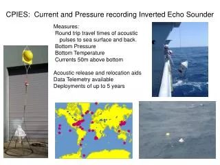
CPIES: Current and Pressure recording Inverted Echo Sounder Measures: Round trip travel times of acoustic pulses to sea surface and back. Bottom Pressure Bottom Temperature Currents 50m above bottom Acoustic release and relocation aids Data Telemetry available Deployments of up to 5 years
Results from PIES & CPIES measurements • One PIES profiles of specific volume anomaly, steric height & mass-loading component SSH ________________________________________________________ • Two PIES / profiles of baroclinic velocity / CPIES plus barotropic referenced velocity = absolute velocity profile 1-D line velocity transect, absolute transports ________________________________________________________ • Three PIES / profiles of baroclinic velocity vector / CPIES plus barotropic velocity vector = absolute velocity vector profile 2-D array 4-D maps of velocity and density structure
Tight empirical relationships exist between acoustic travel time and Fofonoff Potential and Geopotential Anomaly Mass Transport Streamfunction Baroclinic Velocity Streamfunction WOCE SR3 examples, in SAF south of Australia
View the vertical structure of Specific Volume Anomaly, δ, in streamfunction coordinates… When indexed by Φ3000 the δ lookup table looks like this… δ 10-5 kg/m3 Φ3000 (m2 s-1) WOCE SR3 examples, in SAF south of Australia
View the vertical structure of Specific Volume Anomaly, δ, in streamfunction coordinates… When indexed by Φ3000 the δ lookup table looks like this… When indexed by τ3000 the δ lookup table looks like this… δ 10-5 kg/m3 Φ3000 (m2 s-1) τ3000 (s)
Eastward baroclinic transports crossing WOCE SR3 Solid – CTDs (S. Rintoul) Dashed – IES method Transports relative to 3000 dbar
Three IESs, 2-D array: profiles of BC velocity vector SYNOP moored Current Meter measurements and IES’s stack of velocities from Current Meters => stack of velocities from <= IESs (65 km spacing) … differences can be entirely attributed to point sampling vs. lateral-average sampling differences
A CPIES mapping array determines the velocity field as the sum of a baroclinic profile plus barotropic reference velocity The BC velocities are aligned in a single direction (called ‘equivalent barotropic’); adding a BT component can cause turning.
Mesoscale array of PIESs and deep CMs:Abyssal cyclones develop under steep upper-jet troughs • Maps show three fields • Pressure field anomaly at 3500 mIncolor • Depth of the 12°C isotherm contoured ––– at 200 m intervals • Velocity vectors at 3500 m Tick marks: 50 km intervals
Mesoscale array of PIESs and deep CMs:Abyssal cyclones develop under steep upper-jet troughs
Summary • PIES with deep current reference, e.g., CPIES capabilities • 1-D transects provide absolute velocity and transport estimates • Cost-effective for high horizontal spatial resolution • Geostrophic velocities are laterally integrated (intrinsically) • High temporal sampling for extended time periods (up to 5 years) • 2-D arrays of CPIESs can provide velocity structure • With mesoscale spatial and temporal resolution • Well-resolved maps allow for dynamical diagnoses & case-studies
End of planned presentation • Some extra slides follow
IES-estimated temperatures agree with measured temperatures In the Sub-Antarctic Front south of Australia Measured temperatures IES-estimated temperatures
Assemble regional hydrographic data set T (oC) Hydrographic data sorted by tau Choose reference _index Sort hydrographic data by _index … examples from Gulf of Mexico τ
Fit cubic splines to data T (oC) τ
Final GEM field – a lookup table T (oC) τ
Final GEM field – a lookup table T (oC) τ
Three PIES and a deep CM yield profiles of absolute velocity vectors . MMS / SAIC - Gulf of Mexico moorings
IES-estimated currents agree with measured currents In the Sub-Antarctic Front south of Australia Dotted – Measured currents Solid – IES-estimated currents
A CPIES mapping array determines the velocity field as the sum of a baroclinic profile plus barotropic reference velocity The BC velocities are aligned in a single direction (called ‘equivalent barotropic’); adding a BT component can cause turning.
Mapping and case studies, cont’dsteep meander loop, deep eddy field, and RAFOS tracks Tick marks: 50 km apart