Download
1 / 36
360 likes | 472 Vues
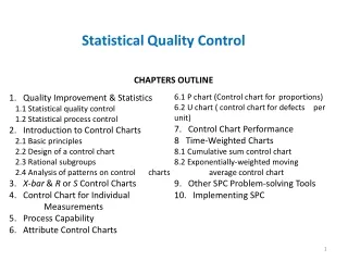
MGS 3100 Business Analysis Statistical Quality Control Oct 17, 2011. Overview. Agenda. Process Capability. Six Sigma. Statistical Process Control.

E N D
MGS 3100Business AnalysisStatistical Quality ControlOct 17, 2011
Overview Agenda Process Capability Six Sigma
Statistical Process Control • Statistical Process Control (SPC) is a statistical procedure using control charts to see if any part of a production process is not functioning properly and could cause poor quality. • In Total Quality Management (TQM) employees use SPC to see if their process is in control – working properly. By continually monitoring the production process and making improvements, the employee contributes to the TQM goal of continuous improvement and few or no defects. • Source: Selected Chapters on Business Analysis – Ch15 Statistical Process Control
Quality Measures – Attributes & Variables • An attribute is a product characteristics such as color, surface texture, cleanliness, or perhaps smell or taste. Attributes can be evaluated quickly with a discrete response such as good or bad, acceptable or not, yes or no. An attribute measure evaluation is sometimes referred to as a qualitative classification, since the response is not measured. • A variable measure is a product characteristics that is measured on a continuous scale such as length, weight, temperature, or time. For example, the amount of liquid detergent in a plastic container can be measured to see if it conforms to the company’s product specifications. • Source: Selected Chapters on Business Analysis – Ch15 Statistical Process Control
Control Charts • Control Charts have historically been used to monitor the quality of manufacturing process. SPC is just as useful for monitoring quality in services. The difference is the nature of the “defect” being measured and monitored. Using Motorola’s definition – a failure to meet customer requirements in any product or service. • Control Charts are graphs that visually show if a sample is within statistical control limits. The control limits are the upper and lower bands of a control chart. They have two basic purposes, to establish the control limits for a process and then to monitor the process to indicate when it is out of control. All control charts look alike, with a line through the center of a graph that indicates the process average and lines above and below the center line that represent the upper and lower limits of the process. • Source: Selected Chapters on Business Analysis – Ch15 Statistical Process Control
Control Charts for Attributes • The quality measures used in attribute control charts are discrete values reflecting a simple decision criterion such as good or bad. A p-chart uses the proportion of defective items in a sample as the sample statistics; a c-chart uses the actual number of defects per item in a sample. • p-charts • Although a p-chart employs a discrete attribute measure (i.e. number of defective items) and thus is not continuous, it is assumed that as the sample size gets larger, the normal distribution can be used to approximate the distribution of the proportion defective. • Source: Selected Chapters on Business Analysis – Ch15 Statistical Process Control Z
Control Charts for Attributes~ p-chart • The p-formula – the sample proportion defective; an estimate of the process average • The standard deviation of the sample proportion • To calculate control limits for the p-chart: • z = the number of standard deviations from the process average. In the control limit formulas for p-charts (and other control charts), z is occasionally equal to 2.00 but most frequently is 3.00. A z value of 2.00 corresponds to an overall normal probability of 95 percent and z = 3.00 corresponds to a normal probability of 99.74 percent. Total defectives Total sample observations k = the number of samples n = the sample size δp = n Z n Z
Control Charts for Attributes~ p-chart (Example) • Please read Example 1 on page 337. • The Western Jeans company produces denim jeans. The company wants to establishes p-chart to monitor the production process and maintain high quality. Western believes that approx. 99.74 percent of the variability in the production process (z = 3.00) is random and thus should be within control limits, whereas 0.26 percent of the process variability is not random and suggests that the process is out of control. • The company has taken 20 samples (one per day for 20-days), each containing 100 pairs of jeans (n=100), and inspected them for defects. The total number of defectives are 200. • Find the control limits. • Source: Selected Chapters on Business Analysis – Ch15 Statistical Process Control Z
Control Charts for Attributes~ c-chart • A c-chart is used when it is not possible to compute a production defective and the actual number of defects must be used. For example, when automobiles are inspected, the number of blemishes (i.e. defects) in the paint job can be counted for each car, but a proportion cannot be computed, since the total number of possible blemishes is not known. • The standard deviation • To calculate control limits for the p-chart: • Please read Example 2 on page 340. • Source: Selected Chapters on Business Analysis – Ch15 Statistical Process Control = the total number of defects / total number of samples f δc = Z Z
Control Charts for Attributes~ c-chart (Example) • Please read Example 2 on page 340. • The Ritz Hotel believes that approximately 99% of the defects (corresponding to 3-sigma limits) are caused by natural, random variations in the housekeeping and room maintenance service, with 1% caused by nonrandom variability. They want to construct a c-chart to monitor the housekeeping service. • 15 inspections samples are selected by the hotel. An inspection sample includes 12 rooms and the total number of defects is 190. • Find the control limits. • Source: Selected Chapters on Business Analysis – Ch15 Statistical Process Control Z
Control Charts for Variables~ R-chart • Variable control charts are for continuous variables that can be measured, such as weight or volume. Two commonly used variable control charts are the range chart (R-chart) and the mean chart (x-bar chart). • R-chart • In an R-chart, the range is the difference between the smallest and largest values in a sample. This range reflects the process variability instead of the tendency toward a mean value. • R is the range of each sample • k is the number of samples. • Source: Selected Chapters on Business Analysis – Ch15 Statistical Process Control Z
Control Charts for Variables~ R-chart (Example) • Please read Example 3 on page 343. • In the production process for a particular slip-ring bearing the employees have taken 10 samples (during 10-day period) of 5 slip-ring bearings (n=5). Please define the control limits for R-chart. The individual observations from each sample are shown as follows: R Z
Control Charts for Variables~ x-bar chart • For an x-bar chart, the mean of each sample is computed and plotted on the chart; the points are sample means. The samples tend to be small, usually around 4 or 5. • n is the sample size (or number of observations) • k is the number of samples • Source: Selected Chapters on Business Analysis – Ch15 Statistical Process Control Z
Control Charts for Variables~ x-bar chart (Example) • Please read Example 4 on page 345. • Use the data from Example 3 and define the control limits for x-bar chart. Z
Control Charts for Variables~ Tabular values for X-bar and R charts (Given)
Control Charts for Variables~ Tabular values for X-bar and R charts (Given)
Agenda Process Capability Six Sigma Overview
Process Capability • Process Capability – A measure of how “capable” the process is to meet customer requirements; compares process limits to tolerance limits. There are three main elements associated with process capability – process variability (the natural range of variation of the process), the process center (mean), and the design specifications. • Process limits (The “Voice of the Process” or The “Voice of the Data”) - based on natural (common cause) variation • Tolerance limits (The “Voice of the Customer”) – customer requirements
(1) (3) specification specification common variation common variation (2) (4) specification specification common variation common variation Process Capability • Variation that is inherent in a production process itself is called common variation.
Process Capability Ratio • One measure of the capability of a process to meet design specifications is the process capability ratio (Cp). It is defined as the ratio of the range of the design specifications (the tolerance range) to the range of process variation, which for most firms is typically ±3δ or 6δ • If Cp is less than 1.0, the process range is greater than the tolerance range, and the process is not capable of producing within the design specifications all the time. If Cp equals 1.0, the tolerance range and the process range are virtually the same. If Cp is greater than 1.0, the tolerance range is greater than the process range. • Companies would logically desire a Cp equal to 1.0 or greater, since this would indicate that the process is capable of meeting specifications.
Process Capability Ratio (Example) • Please read Example 6 on page 354. • The XYZ Snack Food Company packages potato chips in bags. The net weight of the chips in each bag is designed to be 9.0 oz, with a tolerance of +/- 0.5 oz. The packaging process results in bags with an average net weight of 8.80 oz and a standard deviation of 0.12 oz. The company wants to determine if the process is capable of meeting design specifications.
Process Capability Index • The Process Capability Index (Cpk) differs from the Cp in that it indicates if the process mean has shifted away from the design target, and in which direction it has shifted – that is, if it is off center. • If the Cpk index is greater than 1.00 then the process is capable of meeting design specifications. If Cpk is less than 1.00 then the process mean has moved closer to one of the upper or lower design specifications, and it will generate defects. When Cpk equals Cp, this indicates that the process mean is centered on the design (nominal) target. • Please read Example 7 on page 354. • where • x-bar is the mean of the process • sigma is the standard deviation of the process • UTL is the customer’s upper tolerance limit (specification) • and LTL is the customer’s lower tolerance limit
Interpreting the Process Capability Index • Cpk < 1 Not Capable • Cpk > 1 Capable at 3 • Cpk > 1.33 Capable at 4 • Cpk > 1.67 Capable at 5 • Cpk > 2 Capable at 6
Process Capability Index (Example) • A process has a mean of 45.5 and a standard deviation of 0.9. The product has a specification of 45.0 ± 3.0. Find the Cpk .
Process Capability Index (Example) • = min { (45.5 – 42.0)/3(0.9) or (48.0-45.5)/3(0.9) } • = min { (3.5/2.7) or (2.5/2.7) } • = min { 1.30 or 0.93 } = 0.93 (Not capable!) • However, by adjusting the mean, the process can become capable.
Agenda Overview Process Capability Six Sigma
What is Six Sigma? • A goal of near perfection in meeting customer requirements • A sweeping culture change effort to position a company for greater customer satisfaction, profitability and competitiveness • A comprehensive and flexible system for achieving, sustaining and maximizing business success; uniquely driven by close understanding of customer needs, disciplined use of facts, data, and statistical analysis, and diligent attention to managing, improving and reinventing business processes • Source: The Six Sigma Way by Pande, Neuman and Cavanagh
Six Sigma Quality • The objective of Six Sigma quality is 3.4 defects per million opportunities!
Six Sigma Improvement MethodsDMAIC vs. DMADV Define Measure Analyze Continuous Improvement Reengineering Improve Design Control Validate
Six Sigma DMAIC Process- Define • Define: Define who your customers are, and what their requirements are for your products and services – Their expectations. Define your team goals, project boundaries, what you will focus on and what you won’t. Define the process you are striving to improve by mapping the process. Control Improve Define Analyze Measure
Six Sigma DMAIC Process- Measure • Measure: Eliminate guesswork and assumptions about what customers need and expect and how well processes are working. Collect data from many sources to determine speed in responding to customer requests, defect types and how frequently they occur, client feedback on how processes fit their needs, how clients rate us over time, etc. The data collection may suggest Charter revision. Control Improve Define Analyze Measure
Six Sigma DMAIC Process- Analyze • Analyze: Grounded in the context of the customer and competitive environment, analyze is used to organize data and look for process problems and opportunities. This step helps to identify gaps between current and goal performance, prioritize opportunities to improve, identify sources of variation and root causes of problems in the process. Control Improve Define Analyze Measure
Six Sigma DMAIC Process- Improve • Improve: Generate both obvious and creative solutions to fix and prevent problems. Finding creative solutions by correcting root causes requires innovation, technology and discipline. Control Improve Define Analyze Measure
Six Sigma DMADV Process- Design • Design: Develop detailed design for new process. Determine and evaluate enabling elements. Create control and testing plan for new design. Use tools such as simulation, benchmarking, DOE, Quality Function Deployment (QFD), FMECA analysis, and cost/benefit analysis. Validate Design Define Analyze Measure
Six Sigma DMADV Process- Validate • Validate: Test detailed design with a pilot implementation. If successful, develop and execute a full-scale implementation. Tools in this step include: planning tools, flowcharts/other process management techniques, and work documentation. Validate Design Define Analyze Measure