Download
1 / 20
200 likes | 286 Vues
This presentation discusses the sensitivity of surface temperature analyses to background and observation errors. It includes the development of a Local Surface Analysis, case studies, data denial methodology, and results. The research aims to improve the accuracy of high-resolution mesoscale analyses.

E N D
Daniel P. Tyndall and John D. Horel Department of Atmospheric Sciences, University of Utah Salt Lake City, Utah Sensitivity of Surface Temperature Analyses to Background and Observation Errors
Outline • Note: This talk is an excerpt from a paper that has been recently submitted to WAF for review (with M. de Pondeca as a co-author) • Introduction • Research motivation • Goals • Development of a Local (2D-Var) Surface Analysis • Downscaled background • Observations • Specification of observation error variances and background error covariances • Data denial methodology • Hilbert curve withholding technique • Root-mean-square error and sensitivity • Case Study • Shenandoah Valley, morning surface inversion • Results • Summary
Introduction • High resolution mesoscale analyses becoming necessary in variety of fields • Research began in 2006 to help evaluate Real-Time Mesoscale Analysis (RTMA) • Estimate error (co)variances of background and observations • Identify overfitting problems in analyses • Developed a local surface analysis to help meet these goals • Goals of this presentation: • Describe the local surface analysis • Present estimates of the background error covariance and observation error variance • Present a data denial methodology to assess analysis accuracy and identify overfitting problems
Local Surface Analysis (LSA) • 2D-Var surface temperature analysis • Background • 5 km res. downscaled RUC 1-hr forecast • RTMA 5-km terrain developed from NDFD • Observations • Includes various mesonet and METAR observations • ±12 min time window; -30/+12 min time window for RAWS observations • Background and observation errors • Specified in terms of vertical and horizontal spatial distance using decorrelation length scales • Determined using month long sample of observations
Background Downscaling for Temperature • Horizontal bilinear interpolation • Vertical interpolation to height of RTMA terrain using RUC low level lapse rate • RTMA < RUC Elevation: RUC low level lapse rate multiplied by distance between two elevations and added to RUC 2-m temperature • RTMA > RUC Elevation: RUC 2-m temperature used • For complete downscaling description, see Benjamin et al. 2007 • Problem: unphysical features in strong surface temperature inversions
Observation and Background Error Variances • Statistical analysis performed on month-long sample of observations across CONUS • See paper for details; same method used by Myrick and Horel (2006) • Results of analysis show σo2:σb2 should be doubled (2:1)
Background Error Covariance: Example Correlation - Winchester, VA R = 40 km, Z = 100 m R = 80 km, Z = 200 m 0.3 0.4 0 0.1 0.2 0.5 0.6 0.7 0.8 0.9 1.0
Data Denial Methodology • Evaluation of analyses done by randomly withholding observations • Two error measures: • Root-mean-square error (RMSE) calculated at the observation gridpoints • Root-mean-square sensitivity computed across all gridpoints • Measures need observations that are randomly distributed across the grid to be effective
Shenandoah Valley Case Study • 4°x4° area centered over Shenandoah Valley, VA • Shenandoah Valley between Blue Ridge Mtns. And Appalachian Mtns. • Washington, D.C. located in eastern part of domain KIAD Appalachian Mountains Shenandoah Valley Washington, D.C. Blue Ridge Mountains 0 100 200 300 400 500 600 700 800 900 1000
Case Study: Synoptic Situation 1200 UTC 22 October 2007 KIAD • Analyzing analysis generated for 0900 UTC 22 October 2007 • Strong surface inversion up to 1500 m in morning sounding
Case Study: Background Field • Downscaling leads southwest-northwest oriented bands • Observations provide detail along mountain slopes and in Shenandoah Valley 6 2 3 4 5 11 16 17 7 8 9 10 12 13 14 15
Case Study: Observations METAR 16/59/1,744 OTHER 10/75/1,961 PUBLIC 215/575/6,486 RAWS 3/11/1,301
LSA Analyses R = 40 km, Z = 100 m, σo2/σb2 = 1 R = 80 km, Z = 200 m, σo2/σb2 = 2 6 11 16 17 2 3 4 5 8 9 10 12 13 14 15 7
LSA Analysis Increments R = 40 km, Z = 100 m, σo2/σb2 = 1 R = 80 km, Z = 200 m, σo2/σb2 = 2 -3 5 -5 -4 -1 0 1 2 3 4 -2
Data Denial Example • Data denial methodology applied using 10 observation sets • RMSE and Sensitivity computed for each set of analysis characteristics • Right: Difference between control analysis and data withheld analysis • Blue (red) means control analysis was colder (warmer) than withheld 2 -2.5 -2 -1.5 -1 -0.5 0 0.5 1 1.5 2.5
Results Measure of analysis quality in data rich areas Measure of analysis quality in data voids
Summary • Local 2D-Var surface analysis developed for this research • Ratio of observation to background error variance and decorrelation length scales larger than previously assumed • Analysis of RMSE values using withheld observations and all observations provides a measure of analysis overfitting • For further information, see full article submitted to WAF for review
Specification of Observation Error Variance and Background Error Covariance • Statistical analysis using month long sample to estimate error variances • See Myrick and Horel 2006 • Background error covariance specified in terms of spatial distance: • Estimation shows a σo2:σb2 of 2:1 and horiz. and vert. decorrelation length scales of 80 km and 200 m