State Variables
State Variables. Outline. • State variables. • State-space representation. • Linear state-space equations. • Nonlinear state-space equations. • Linearization of state-space equations. Input-output Description. The description is valid for

State Variables
E N D
Presentation Transcript
Outline • State variables. • State-space representation. • Linear state-space equations. • Nonlinear state-space equations. • Linearization of state-space equations.
Input-output Description The description is valid for a) time-varying systems: ai, cj, explicit functions of time. b) multi-input-multi-output (MIMO) systems: l input-output differential equations, l = # of outputs. c) nonlinear systems: differential equations include nonlinear terms.
State Variables To solve the differential equation we need (1) The system input u(t) for the period of interest. (2) A set of constant initial conditions. • Minimal set of initial conditions: incomplete knowledge of the set prevents complete solution but additional initial conditions are not needed to obtain the solution. • Initial conditions provide a summary of the History of the system up to the initial time.
Definitions System State: minimal set of numbers {xi(t), i = 1,2,...,n}, needed together with the input u(t), t ∈ [t0,tf) to uniquely determine the behavior of the system in the interval [t0,tf]. n = order of the system. State Variables: As t increases, the state of the system evolves and each of the numbers xi(t) becomes a time variable. State Vector: vector of state variables
Notation • Column vector bolded • Row vector bolded and transposed xT.
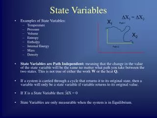
Definitions State Space: n-dimensional vector space where {xi(t), i = 1,2,...,n} represent the coordinate axes State plane: state space for a 2nd order system Phase plane: special case where the state variables are proportional to the derivatives of the output. Phase variables: state variables in phase plane. State trajectories: Curves in state space State portrait: plot of state trajectories in the plane (phase portrait for the phase plane).
Example 7.1 • State for equation of motion of a point mass m driven by a force f • y = displacement of the point mass. 2 ⇒ system is second order
Example 7.1 State Equations State variables State vector 2 Phase Variables: 2nd = derivative of the first. Two first order differential equations 1. First equation: from definitions of state variables. 2. Second equation: from equation of motion.
Solution of State Equations Solve the 1st order differential equations then substitute in y = x1 2 differential equations + algebraic expression are equivalent to the 2nd order differential equation. Feedback Control Law 2nd order underdamped system u /m = −3x −9x 1. Solution depends only on initial conditions. 2. Obtain phase portrait using MATLAB command lsim, 3. Time is an implicit parameter. 4. Arrows indicate the direction of increasing time. 5. Choice of state variables is not unique.
State Equations • Set of first order equations governing the state variables obtained from the input-output differential equation and the definitions of the state variables. • In general, n state equations for a nth order system. • The form of the state equations depends on the nature of the system (equations are time-varying for time-varying systems, nonlinear for nonlinear systems, etc.) • State equations for linear time-invariant systems can also be obtained from their transfer functions.
Output Equation • Algebraic equation expressing the output in terms of the state variables. • Multi-output systems: a scalar output equation is needed to define each output. • Substitute from solution of state equation to obtain output.
State-space Representation • Representation for the system described by a differential equation in terms of state and output equations. • Linear Systems: More convenient to write state (output) equations as a single matrix equation
Example 7.2 • The state-space equations for the system of Ex. 7.1
Linear Vs. Nonlinear State-Space Example 7.3: The following are examples of state-space equations for linear systems a) 3rd order 2-input-2-output (MIMO) LTI
Example 7.3 (b) 2nd order 2-output-1-input (SIMO) linear time-varying 1. Zero direct D, constant B and C. 2. Time-varying system: A has entries that are functions of t.
Example 7.4: Nonlinear System Obtain a state-space representation for the s-D.O.F. robotic manipulator from the equations of motion with output q.
Solution order 2 s (need 2 s initial conditions to solve completely. State Variables
Example 7.5 Write the state-space equations for the 2- D.O.F. anthropomorphic manipulator.
Nonlinear State-space Equations f(.) (n×1) and g(.) (l ×1) = vectors of functions satisfying mathematical conditions to guarantee the existence and uniqueness of solution. affine linear in the control: often encountered in practice (includes equations of robotic manipulators)
Linearization of State Equations • Approximate nonlinear state equations by linear state equations for small ranges of the control and state variables. • The linear equations are based on the first order approximation. x0 constant, Δx= x - x0 = perturbation x0 . Approximation Error of order Δ2x Acceptable for small perturbations.
Example 7.6 Motion of nonlinear spring-mass-damper. y = displacement f = applied force m = mass of 1 Kg b(y) = nonlinear damper constant k(y) = nonlinear spring force. Find the equilibrium position corresponding to a force f0 in terms of the spring force, then linearize the equation of motion about this equilibrium.
Solution Equilibrium of the system with a force f0 (set all the time derivatives equal to zero and solve for y) Equilibrium is at zero velocity and the position y0.
Linearize about the equilibrium • Entries of state matrix: constants whose values depend on the equilibrium. • Originally linear terms do not change with linearization.