
Learning Curves in Cost Estimation: Theories and Applications
E N D
Presentation Transcript
Learning Curve Introduction • Learning Curves are used to estimate the time saving that is experienced when performing the same task multiple times • The greater the amount of labour involved in the task, the greater the saving experienced with each iteration
Learning Curve Introduction • Clearly manufacturing a ship or airline has a steeper learning curve (greater savings per iteration) than an automated process of making widgets (e.g. previous figure which is steep - ships) • Two predominant learning curve theories (though there are more) • Unit Theory • Cumulative Average Theory • Both will be explained using the Canadian Frigate program from the late 1980s and early 1990s
Unit Theory Learning Curve • The theory states that the cost decreases by a fixed percentage as the quantity produced doubles • The following table reflects an 80% learning curve which means the cost decreases by 20% for each doubling of production (multiply by .8) Note: Examples from Cost Estimation by Mislick and Nussbaum
Unit Theory Learning Curve • Unit Theory equation • Yx = A * xbwhere: • Yx = the cost of unit x • A = cost of the first unit • x = the unit number • s = the slope of the learning curve = 2b • Cost of 2x = (cost of x)*s • Substituting A*xb for cost & rearrange • s = A*(2x)b/A*xb = 2b • Using logarithms: b = ln(s)/ln(2)
Unit Theory Learning Curve • From the previous example: • A=100 • Slope of learning curve = 0.8 • 0.8 = 2b • Using logarithms: • ln(0.8) = b * ln(2) • b = ln(0.8)/ln(2) = -0.3219 • Therefore, cost unit x = 100 * x -0.3219 • For x = 4, cost = 64.0 • For x =3, cost = 70.2
Unit Theory Learning Curve • Canadian Frigate Example
Unit Theory Learning Curve • Yx = A * xb • To determine “b”, use logarithms, i.e. • ln(Yx) = ln(A) + b*ln(x) • “b” slope of this equation (learning slope = 2b) • Graph using Excel Scatter with Markers after converting your costs (hours in this case) and number of units using natural logs • Under Chart Tools, select Trendline– more trendline options • Then select display equation on chart and display R-squared value on chart
Unit Theory Learning Curve • From the chart equation, the slope is -0.4482 which = b • From before, if s = 2b, then s = 0.7330 or a 73.3% unit learning curve which is steeper than typical but reasonable given SJSL’s inexperience
Cumulative Average Theory • Subtly different from Unit Theory • Cumulative average theory is average cost of groups of units while unit theory is based on individual unit cost • Therefore, for cumulative average theory (using the previous 80% example): • The average cost of 2 units is 80% of 1 unit • The average cost of 4 units is 80% of 2 units • The average cost of 50 units is 80% of 25 units • Doubling your production reduces your average cost by your learning curve (80% for this example)
Cumulative Average Theory • Cumulative Average Theory equation • YN= A * Nbwhere: • YN= the cumulative average cost of N units • A = cost of the first unit • N = the cumulative number of units produced • As before: • s = the slope of the learning curve = 2b • Using logarithms: b = ln(s)/ln(2) • Cumulative Average Theory usually used for production lots where batches of units are made
Cumulative Average Theory • Canadian Frigate example again:
Cumulative Average Theory • From the chart equation, the slope is -0.2244 which = b • From before, if s = 2b, then s = 0.8560 or a 85.6% unit learning curve which is less steep than unit theory as expected
Unit vs Cumulative Average Theory • Cumulative average theory is a less steep curve such that unit learning is always below it • Cumulative average is less responsive to variation in costs from unit to unit since it is based on averages • Use cumulative if initial production is expected to have large cost variation unit to unit
Unit vs Cumulative Average Theory • For Frigate example, which learning curve is better? • Hard to tell visually, I used stats, went with unit • R2 for unit = 0.9562 vs cumulative = 0.9355 • P-value (not shown) unit=5.2x10⁻⁶ cum=2.0x10⁻⁵