Download
1 / 35
1.95k likes | 3.69k Vues
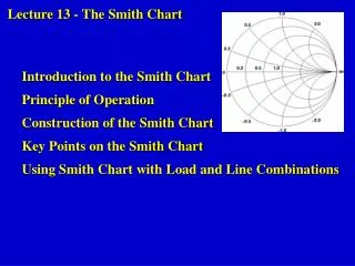
Lecture 13 - The Smith Chart Introduction to the Smith Chart Principle of Operation Construction of the Smith Chart Key Points on the Smith Chart Using Smith Chart with Load and Line Combinations. THE SMITH CHART.

E N D
Lecture 13 - The Smith Chart Introduction to the Smith Chart Principle of Operation Construction of the Smith Chart Key Points on the Smith Chart Using Smith Chart with Load and Line Combinations
THE SMITH CHART • Devised in 1944 by Philip H. Smith, Bell Labs, U.S.A. • A graphical aid for transmission line calculations. • Used nowadays for designing “matching” circuits and displaying RF data. Philip Smith: 1905-1987
l ZL Load Transmission line, Zo Generator The Smith Chart basically enables you to convert between and Z graphically, either at the load or at an arbitrary point down the line.
Simplified Smith Chart 1 In this simplified version of the Smith Chart most of the grid of lines has been removed. For clarity, in these lectures this version will be used to illustrate the properties of the Smith Chart. 0.5 2 3 0.2 5 10 0 0.2 0.5 1 2 3 5 10 0 -10 -5 -0.2 -3 -2 -0.5 -1
Simplified Smith Chart 1 In this simplified version of the Smith Chart most of the grid of lines has been removed. For clarity, in these lectures this version will be used to illustrate the properties of the Smith Chart. 0.5 2 3 0.2 5 10 0 0.2 0.5 1 2 3 5 10 0 -10 -5 -0.2 -3 -2 -0.5 -1
SMITH CHART BASICS • ρis a complex quantity: ρ= |ρ|e jφ • For all ZL, 0 <|ρ| <1 Circle of UNIT RADIUS in complex number plane Imaginary +jX R+jX φ |ρ| (1,0) 0 R Real -jX Complex Impedance Plane Complex Reflection Coefficient Plane
ρZL To avoid having to use a different Smith Chart for every value of Zo, the normalised impedance, z , is used: z = ZL/ Zo The normalised impedance z can then be “denormalised” to obtain the load impedance ZL by multiplying by Zo: ZL = z.Zo In terms of its real and imaginary components, the normalised impedance can be written as: z = r + jx
CONSTRUCTION OF THE SMITH CHART (pages 3-5) is for information only IT IS NOT EXAMINABLE
MAPPING BETWEEN IMPEDANCE PLANE AND THE SMITH CHART r is the normalised resistance axis x is the normalised reactance axis Lines of constant normalised resistance Lines of constant normalised reactance r = 0 1 0.5 2 0.4 0.2 0 -0.2 -0.4 x = X/Zo 3 0.2 5 x = 0 10 x r = R/Zo 0 0.2 0.5 1 2 3 5 10 r 0.2 0.4 0.6 0.8 0 -10 -5 -0.2 -3 -2 -0.5 Complex (Normalised) Impedance Plane -1 Smith Chart
1 0.5 2 3 0.2 5 10 x 0 0.2 0.5 1 2 3 5 10 0 r -10 -5 -0.2 -3 -2 -0.5 -1 normalised reactance, x normalised resistance, r
0.70745º 0.707 45º 1/0º Step 1: Plot ρ Example (page 2): Measurements on a slotted line with Zo = 50Ω give: |ρ| = 0.707 and φ= 45º. Find ZL ρ Unit Circle in Reflection Coefficient Plane
1 0.5 2 3 0.70745º 0.2 5 0.707 10 x 0 0.2 0.5 1 2 3 5 10 0 45º r 1/0º -10 -5 -0.2 -3 -2 -0.5 -1 Step 2: Superimpose Smith Chart grid Example (page 2): Measurements on a slotted line with Zo = 50Ω give: |ρ| = 0.707 and φ= 45º. Find ZL Unit Circle in Reflection Coefficient Plane
Step 3: Read off normalised values for r and x 1 0.5 2 3 0.707/45º 0.2 5 0.707 10 x 0 0.2 0.5 1 2 3 5 10 0 45º r 1/0º -10 -5 -0.2 -3 -2 -0.5 -1 Example (page 2): Measurements on a slotted line with Zo = 50Ω give: |ρ| = 0.707 and φ= 45º. Find ZL , x = 2 r = 1 Unit Circle in Reflection Coefficient Plane
1 0.5 2 3 0.70745º 0.2 5 0.707 10 x 0 0.2 0.5 1 2 3 5 10 0 45º r 10º -10 -5 -0.2 -3 -2 -0.5 -1 Step 4: Calculate R and X by “denormalizing”: ZL = Zo(r + jx) = 50(1+j2) = 50 + j100Ω Example (page 2): Measurements on a slotted line with Zo = 50Ω give: |ρ| = 0.707 and φ= 45º. Find ZL , x=2 r=1 Unit Circle in Reflection Coefficient Plane
KEY POINTS ON THE SMITH CHART Open Circuit (ZL = ∞, z = ZL/Zo = ∞) z = r + jx = ∞ 1 0.5 2 ρ= 1/0º ρ= 1/0º 3 0.2 5 10 x 1/0º 0 0.2 0.5 1 2 3 5 10 r 0 -10 -5 -0.2 -3 -2 -0.5 -1 Reflection Coefficient Plane Smith Chart
Short Circuit (ZL = 0, z = 0) 1 0.5 2 3 0.2 5 10 x 10 0 0.2 0.5 1 2 3 5 10 r 0 -10 -5 -0.2 -3 ρ= 1/180º -2 -0.5 ρ= 1/180º z = r + jx = 0 + j0 -1 Reflection Coefficient Plane Smith Chart
Matched Load (ZL = Zo, z = 1) 1 0.5 2 3 0.2 5 10 x 1/0 0 0.2 0.5 1 2 3 5 10 r 0 -10 -5 -0.2 -3 ρ= 0 -2 -0.5 ρ= 0 z = r + jx = 1 + j0 -1 Reflection Coefficient Plane Smith Chart
Resistive Load (ZL = R + j0 , z = r) R and Zo (for a lossless line) are REAL, therefore is real. R > Zo,ρ +ve, φ= 0º R < Zo,ρ -ve, φ= 180º 1 0.5 2 3 0.2 5 10 x R < Zo R = Zo R > Zo 10 0 0.2 0.5 1 2 3 5 10 R = 0 r 0 -10 R = -5 -0.2 -3 -2 -0.5 -1 Reflection Coefficient Plane Smith Chart
Purely Reactive Load (ZL = 0 + jX , z = 0 + jx) 1 0.5 2 3 z = jx (inductive) 0.2 5 10 x 10 0 0.2 0.5 1 2 3 5 10 z = j0 r 0 -10 z = j -5 -0.2 -3 z = jx (capacitive) -2 -0.5 -1 Reflection Coefficient Plane Smith Chart
Purely Reactive Load (ZL = 0 + jX , z = 0 + jx) 1 0.5 2 3 z = jx (inductive) 0.2 5 10 x 10 0 0.2 0.5 1 2 3 5 10 z = j0 r 0 -10 z = j -5 -0.2 -3 z = jx (capacitive) -2 -0.5 -1 Reflection Coefficient Plane Smith Chart
General Case (ZL = R + jX) 1 0.5 2 3 0.2 5 |ρ| 10 φ x 1/0 0 0.2 0.5 1 2 3 5 10 r 0 -10 -5 -0.2 -3 -2 -0.5 -1 Reflection Coefficient Plane Smith Chart
Pure Reactance 1 Pure Resistance 0.5 2 3 0.2 5 Matched Load 10 x 0 0.2 0.5 1 2 3 5 10 0 r -10 Short Circuit Open Circuit -5 -0.2 -3 -2 -0.5 -1
RATIO OF V-/V+ AT AN ARBITRARY DISTANCE l FROM THE LOAD ZL Zo ZL x = -l x = 0 If the line is losslessgl = jbl , hence: r-l= re-2gl= re-j2bl= |r|ejf e-j2bl= |r|ej(f- 2bl) i.e. the magnitude of the reflection coefficient at x = -lis the same as at x = 0 but its phase changes fromfto f - 2bl . An additional phase change of -2blhas been added by the introduction of the length of line,l .
l ZL Load Transmission line Generator 1 0.5 2 3 z = r+jx ρof ZL only 0.2 5 |ρ| φ 10 x 2βl 1/0 0 0.2 0.5 1 2 3 5 10 2βl r 0 -10 -5 ρof ZL plus line of length l -0.2 z of load and line of length l -3 -2 -0.5 Point rotates clockwise by 2βlradians (2x360xl/λ degrees) at a constant radius -1 Reflection Coefficient Plane Smith Chart
In the case of a lossless line a = 0, so g = a + jb = jb and is purely imaginary, so the hyperbolic functions reduce to trigonometric functions: Zin becomes: or: Original expression:
l ZL “Clockwise towards generator” Load Transmission line Generator 1 0.5 2 3 z = r+jx of ZL only 0.2 5 |ρ| φ 10 x 2βl 1/0 0 0.2 0.5 1 2 3 5 10 2βl r 0 -10 -5 of ZL plus line of length l -0.2 z of load and line of length l -3 -2 -0.5 -1 Point rotates clockwise by 2βl radians (2x360 l/λ degrees) Reflection Coefficient Plane Smith Chart
Tutorial C, Question 2 Solution by Smith Chart To find Zin: • zL = ZL/Zo • = (100+j50)/75 • = 1.33+j0.67 zL 3. 2l = 2x2l/λ = 2x2fl/v = 1.26 radians = 72º 4. Read z-l from chart: z-l = 1.75-j0.45 72º 2. Plot zL on Smith Chart z-l 5. Denormalise to find Zin: Zin = Zo x z-l = 75(1.75-j0.45) = 131-j34 Ω (cf. 126-j36 Ω by exact calculation) Zo = 75 Ω ZL = 100 + j50 Ω l = 2.2 m, f = 100 MHz v = 2 x 10⁸ ms-1
For extra copies of the Smith Chart go to the Web page for my part of the course and click on the Smith Chart link
The Smith Chart & General Transmission Lines r-l = re-2gl = re-2αle-j2bl = |r|ejf e-2αl e-j2bl = |r|e-2αlej(f-2bl) = +j - propagation constant - attenuation constant - phase constant 1 0.5 2 z = r+jx ρ 3 0.2 5 10 x 10 0 0.2 0.5 1 2 3 5 10 r 0 ρ-l -10 z of load and line of length l -5 -0.2 -3 -2 -0.5 -1 Reflection Coefficient Plane Smith Chart
The Smith Chart and Variation of Frequency r-l = |r|ej(φ-2bl)for a lossless line rotation angle is -2l= -2.(2/λ).l = -2.(2.f/v).l = -4fl/v or constant x f 1 0.5 2 ρdc zdc 3 zf1 ρf1 0.2 5 10 x 1/0 0 0.2 0.5 1 2 3 5 10 ρf2 r 0 zf2 -10 -5 -0.2 ρf3 zf3 -3 -2 -0.5 frequency f3 > f2 > f1 -1 Reflection Coefficient Plane Smith Chart
Summary The Smith Chart is used as a graphical aid for converting between a load impedance, Z, and a reflection coefficient,ρ. (This can be done with or without sections of line being present.) ρZL
To avoid having to use a different Smith Chart for every value of Zo, the normalised impedance, z, is used: • z = ZL/Zo • (z = r + jx) • z can then be denormalised to obtain the load impedance ZL, by multiplying by Zo: • ZL = z.Zo
The circles correspond to lines of constant normalised resistance, r. • The arcs correspond to lines of constant normalised reactance, x. r = 0 1 0.5 2 0.4 0.2 0 -0.2 -0.4 x = X/Zo 3 0.2 5 x = 0 10 x r = R/Zo 0 0.2 0.5 1 2 3 5 10 r 0.2 0.4 0.6 0.8 0 -10 -5 -0.2 -3 -2 -0.5 -1 Complex Impedance Plane Smith Chart
Adding a length, l, of lossless line to a load, ZL, corresponds on the Smith Chart to rotating at constant radius from zLCLOCKWISE through an angle 2l. (“CLOCKWISE TOWARDS GENERATOR”) • If the line is not lossless, the radius decreases as we rotate around the centre. • Increasing the signal frequency causes z-l to rotate clockwise around Smith Chart at constant radius.