
Understanding Histograms: Construction, Interpretation, and Common Shapes
E N D
Presentation Transcript
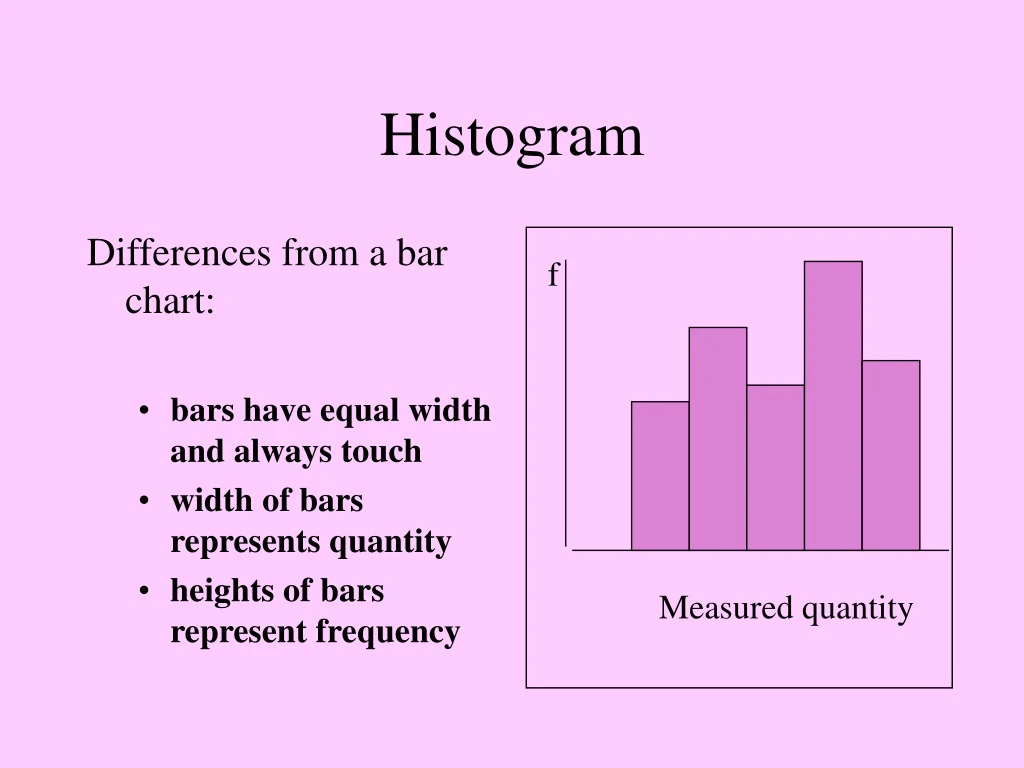
Histogram Differences from a bar chart: • bars have equal width and always touch • width of bars represents quantity • heights of bars represent frequency f Measured quantity
To construct a histogram from raw data: • Decide on the number of classes (5 to 15 is customary). • Find a convenient class width. • Organize the data into a frequency table. • Find the class midpoints and the class boundaries. • Sketch the histogram.
Finding class width 1. Compute: 2. Increase the value computed to the next highest whole number
Raw Data: 10.2 18.7 22.3 20.0 6.3 17.8 17.1 5.0 2.4 7.9 0.3 2.5 8.5 12.5 21.4 16.5 0.4 5.2 4.1 14.3 19.5 22.5 0.0 24.7 11.4 Use 5 classes. 24.7 – 0.0 5 = 4.94 Round class width up to 5. Class Width
Frequency Table • Determine class width. • Create the classes. May use smallest data value as lower limit of first class and add width to get lower limit of next class. • Tally data into classes. • Compute midpoints for each class. • Determine class boundaries.
Tallying the Data # of miles tally frequency 0.0 - 4.9 |||| | 6 5.0 - 9.9 |||| 5 10.0 - 14.9 |||| 4 15.0 - 19.9 |||| 5 20.0 - 24.9 |||| 5
Grouped Frequency Table # of miles f 0.0 - 4.9 6 5.0 - 9.9 5 10.0 - 14.9 4 15.0 - 19.9 5 20.0 - 24.9 5 Class limits: lower - upper
Computing Class Width difference between the lower class limit of one class and the lower class limit of the next class
Finding Class Widths # of miles f class widths 0.0 - 4.9 6 5 5.0 - 9.9 6 5 10.0 - 14.9 4 5 15.0 - 19.9 5 5 20.0 - 24.9 5 5
Computing Class Midpoints lower class limit + upper class limit 2
Finding Class Midpoints # of miles f class midpoints 0.0 - 4.9 6 2.45 5.0 - 9.9 5 10.0 - 14.9 4 15.0 - 19.9 5 20.0 - 24.9 5
Finding Class Midpoints # of miles f class midpoints 0.0 - 4.9 6 2.45 5.0 - 9.9 5 7.45 10.0 - 14.9 4 15.0 - 19.9 5 20.0 - 24.9 5
Finding Class Midpoints # of miles f class midpoints 0.0 - 4.9 6 2.45 5.0 - 9.9 5 7.45 10.0 - 14.9 4 12.45 15.0 - 19.9 5 17.45 20.0 - 24.9 5 22.45
Class Boundaries (Upper limit of one class + lower limit of next class) divided by two
Finding Class Boundaries # of miles f class boundaries 0.0 - 4.9 6 5.0 - 9.9 5 4.95 - 9.95 10.0 - 14.9 4 15.0 - 19.9 5 20.0 - 24.9 5
Finding Class Boundaries # of miles f class boundaries 0.0 - 4.9 6 5.0 - 9.9 5 4.95 - 9.95 10.0 - 14.9 4 9.95 - 14.95 15.0 - 19.9 5 20.0 - 24.9 5
Finding Class Boundaries # of miles f class boundaries 0.0 - 4.9 6 5.0 - 9.9 5 4.95 - 9.95 10.0 - 14.9 4 9.95 - 14.95 15.0 - 19.9 5 14.95 - 19.95 20.0 - 24.9 5
Finding Class Boundaries # of miles f class boundaries 0.0 - 4.9 6 ?? 5.0 - 9.9 5 4.95 - 9.95 10.0 - 14.9 4 9.95 - 14.95 15.0 - 19.9 5 14.95 - 19.95 20.0 - 24.9 5 19.95 - 24.95
Finding Class Boundaries # of miles f class boundaries 0.0 - 4.9 6 ?? - 4.95 5.0 - 9.9 5 4.95 - 9.95 10.0 - 14.9 4 9.95 - 14.95 15.0 - 19.9 5 14.95 - 19.95 20.0 - 24.9 5 19.95 - 24.95
Finding Class Boundaries # of miles f class boundaries 0.0 - 4.9 6 0.05 - 4.95 5.0 - 9.9 5 4.95 - 9.95 10.0 - 14.9 4 9.95 - 14.95 15.0 - 19.9 5 14.95 - 19.95 20.0 - 24.9 5 19.95 - 24.95
6 5 4 3 2 1 0 - - - - - - - | | | | | | -0.05 4.95 9.95 14.95 19.95 24.95 mi. Constructing the Histogram f # of miles f 0.0 - 4.9 6 5.0 - 9.9 5 10.0 - 14.9 4 15.0 - 19.9 5 20.0 - 24.9 5
Relative Frequency Relative frequency = f = class frequency n total of all frequencies
Relative Frequency f = 6 = 0.24 n 25 f = 5 = 0.20 n 25
.24 .20 .16 .12 .08 .04 0 - - - - - - - Relative frequency f/n | | | | | | -0.05 4.95 9.95 14.95 19.95 24.95 mi. Relative Frequency Histogram # of miles f relative frequency 0.0 - 4.9 6 0.24 5.0 - 9.9 5 0.20 10.0 - 14.9 4 0.16 15.0 - 19.9 5 0.20 20.0 - 24.9 5 0.20
Common Shapes of Histograms When folded vertically, both sides are (more or less) the same. Symmetrical f
Common Shapes of Histograms Also Symmetrical f
Common Shapes of Histograms Uniform f
Common Shapes of Histograms Non-Symmetrical Histograms These histograms areskewed.
Common Shapes of Histograms Skewed Histograms Skewedleft Skewed right
Common Shapes of Histograms Bimodal f The two largest rectangles are approximately equal in height and are separated by at least one class.
Frequency Polygon A frequency polygon or line graph emphasizes the continuous rise or fall of the frequencies.
Constructing the Frequency Polygon • Dots are placed over the midpoints of each class. • Dots are joined by line segments. • Zero frequency classes are included at each end.
Constructing the Frequency Polygon Weights (in pounds) f 2 - 4 6 5 - 7 5 8 - 10 4 11 - 13 5 f 6 5 4 3 2 1 0 - - - - - - - | | | | | | 0 3 6 9 12 15 pounds
Cumulative Frequency The sum of the frequencies for that class and all previous or later classes
Cumulative Frequency Table Weights (in pounds) f Greater than 1.5 20 Greater than 4.5 14 Greater than 7.5 9 Greater than 10.5 5 Greater than 13.5 0 Weights (in pounds) f 2 - 4 6 5 - 7 5 8 - 10 4 11 - 13 5 20
Ogive Graph of a cumulative frequency table
Constructing the Ogive Weights (in pounds) f Greater than 1.5 20 Greater than 4.5 14 Greater than 7.5 9 Greater than 10.5 5 Greater than 13.5 0 20 15 10 5 0 - - - - - Cumulative frequency | | | | | | 1.5 4.5 7.5 10.5 13.5 pounds
Exploratory Data Analysis • A field of statistical study useful in detecting patterns and extreme data values • Tools used include histograms and stem-and-leaf displays