Exponential Functions

1. Exponential Functions Define an exponential function. Graph exponential functions. Use transformations on exponential functions. Define simple interest. Develop a compound interest formula. Understand the number e. SECTION 4.1 1 2 3 4 5 6

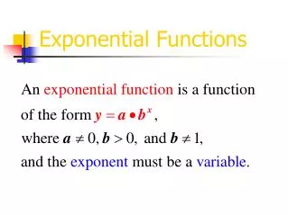
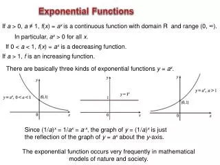
2. EXPONENTIAL FUNCTION A function f of the form is called an exponential function with base a. Its domain is (–∞, ∞).

3. EXAMPLE 1 Evaluating Exponential Functions d. Let F(x) = 4x. Find F(3.2).

4. Solution EXAMPLE 1 Evaluating Exponential Functions d. F(3.2) = 43.2≈ 84.44850629

5. RULES OF EXPONENTS Let a, b, x, and y be real numbers with a > 0 and b > 0. Then

6. Solution Make a table of values. Graphing an Exponential Function with Base a > 1 – Exponential Growth EXAMPLE 2 Graph the exponential function Plot the points and draw a smooth curve.

7. Graphing an Exponential Function with Base a > 1 EXAMPLE 2 Solution continued This graph is typical for exponential functions when a > 1.

8. Solution Make a table of values. Graphing an Exponential Function with Base 0 < a < 1 – Exponential Decay EXAMPLE 3 Sketch the graph of Plot the points and draw a smooth curve.

9. Graphing an Exponential Function with Base 0 < a < 1 EXAMPLE 3 Solution continued As x increases in the positive direction, y decreases towards 0.

10. PROPERTIES OF EXPONENTIAL FUNCTIONS Let f (x) = ax, a > 0, a ≠ 1. 1. The domain of f (x) = ax is (–∞, ∞). 2. The range of f (x) = ax is (0, ∞); the entire graph lies above the x-axis. 3. For a > 1, Exponential Growth (i)f is an increasing function, so the graph rises to the right. (ii) as x → ∞, y→ ∞. (iii) as x → –∞, y → 0.

11. 4. For 0 < a < 1, - Exponential Decay (i)f is a decreasing function, so the graph falls to the right. (ii) as x → – ∞, y→ ∞. (iii) as x → ∞, y → 0. 5. The graph of f (x) = ax has no x-intercepts, so it never crosses the x-axis. No value of x will cause f (x) = ax to equal 0. 6. The graph of is a smooth and continuous curve, and it passes through the points 7. The x-axis is a horizontal asymptote for every exponential function of the form f (x) = ax.

12. TRANSFORMATIONS ON EXPONENTIAL FUNCTION f (x) = ax Vertical Shift y = ax + b Shift the graph of y = ax, |b| units up if b > 0. down if b < 0. Transformation Equation Effect on Equation Horizontal Shift y = ax+b Shift the graph of y = ax, |b| units left if b > 0. right if b < 0.

13. TRANSFORMATIONS ON EXPONENTIAL FUNCTION f (x) = ax Transformation Equation Effect on Equation Stretching or Compressing (Vertically) y = cax Multiply the y coordinates by c. The graph of y = ax is vertically stretched if c > 1. compressed if 0 < c < 1.

14. TRANSFORMATIONS ON EXPONENTIAL FUNCTION f (x) = ax Transformation Equation Effect on Equation Reflection y = –ax Reflect the graph of y = ax in the x-axis. y = a–x Reflect the graph of y = ax in the y-axis.

15. EXAMPLE 6 Sketching Graphs Use transformations to sketch the graph of each function. State the domain and range of each function and the horizontal asymptote of its graph.

16. EXAMPLE 6 Sketching Graphs Solution Domain: (–∞, ∞) Range: (–4, ∞) Horizontal Asymptote: y = –4

17. EXAMPLE 6 Sketching Graphs Solution continued Domain: (–∞, ∞) Range: (0, ∞) Horizontal Asymptote: y = 0

18. EXAMPLE 6 Sketching Graphs Solution continued Domain: (–∞, ∞) Range: (–∞, 0) Horizontal Asymptote: y = 0

19. EXAMPLE 6 Sketching Graphs Solution continued Domain: (–∞, ∞) Range: (–∞, 2) Horizontal Asymptote: y = 2

20. General Exponential Growth/Decay Model Rate of decay (r < 0),Growth (r > 0) Amount after t time periods Number of time periods Original amount

21. COMPOUND INTEREST – Growth Compound interest is the interest paid on both the principal and the accrued (previously earned) interest. It is an application of exponential growth. Interest that is compounded annually is paid once a year. For interest compounded annually, the amount A in the account after t years is given by Rate of decay (r < 0),Growth (r > 0) Amount after t time periods Number of time periods Original amount

22. EXAMPLE 2 Calculating Compound Interest Juanita deposits $8000 in a bank at the interest rate of 6% compounded annually for five years. How much money will she have in her account after five years? b. How much interest will she receive?

23. Solution a. Here P = $8000, r = 0.06, and t = 5. EXAMPLE 2 Calculating Compound Interest b. Interest = AP = $10,705.80  $8000 = $2705.80.

24. COMPOUND INTEREST FORMULA A = amount after t years P = principal r = annual interest rate (expressed as a decimal) n = number of times interest is compounded each year t = number of years

25. Using Different Compounding Periods to Compare Future Values EXAMPLE 3 If $100 is deposited in a bank that pays 5% annual interest, find the future value A after one year if the interest is compounded annually. semiannually. quarterly. monthly. daily.

26. Solution In the following computations, P = 100, r=0.05 and t = 1. Only n, the number of times interest is compounded each year, changes. Since t = 1, nt = n(1) = n. Using Different Compounding Periods to Compare Future Values EXAMPLE 3 (i) Annual Compounding:

27. Using Different Compounding Periods to Compare Future Values EXAMPLE 3 (ii) Semiannual Compounding: (iii) Quarterly Compounding:

28. Using Different Compounding Periods to Compare Future Values EXAMPLE 3 (iv) Monthly Compounding: (v) Daily Compounding:

29. EXAMPLE 8 Bacterial Growth A technician to the French microbiologist Louis Pasteur noticed that a certain culture of bacteria in milk doubles every hour. If the bacteria count B(t) is modeled by the equation with t in hours, find the initial number of bacteria, the number of bacteria after 10 hours; and the time when the number of bacteria will be 32,000.

30. EXAMPLE 8 Bacterial Growth Solution a. Initial size c. Find t when B(t) = 32,000 After 4 hours, the number of bacteria will be 32,000.

31. THE VALUE OF e As h gets larger and larger, gets closer and closer to a fixed number. This irrational number is denoted by e and is sometimes called the Euler number. The value of e to 15 places is e = 2.718281828459045.

32. CONTINUOUS COMPOUND FORMULA A = amount after t years P = principal r = annual rate (expressed as a decimal) t = number of years

33. Solution P = $8300 and r = 0.075. Convert eight years and three months to 8.25 years. EXAMPLE 4 Calculating Continuous Compound Interest Find the amount when a principal of $8300 is invested at a 7.5% annual rate of interest compounded continuously for eight years and three months.

34. Solution a. With simple interest, EXAMPLE 5 Calculating the Amount of Repaying a Loan How much money did the government owe DeHaven’s descendants for 213 years on a $450,000 loan at the interest rate of 6%?

35. EXAMPLE 5 Calculating the Amount of Repaying a Loan Solution continued b. With interest compounded yearly, c. With interest compounded quarterly,

36. EXAMPLE 5 Calculating the Amount of Repaying a Loan Solution continued d. With interest compounded continuously, Notice the dramatic difference between quarterly and continuous compounding and the dramatic difference between simple interest and compound interest.

37. THE NATURAL EXPONENTIAL FUNCTION The exponential function with base e is so prevalent in the sciences that it is often referred to as the exponential function or the natural exponential function.

38. EXAMPLE 6 Sketching a Graph Use transformations to sketch the graph of Solution Start with the graph of y = ex.

39. EXAMPLE 6 Sketching a Graph Use transformations to sketch the graph of Solution coninued Shift the graph of y = ex one unit right.

40. EXAMPLE 6 Sketching a Graph Use transformations to sketch the graph of Solution continued Shift the graph of y = ex – 1 two units up.

41. MODEL FOR EXPONENTIALGROWTH OR DECAY A(t) = amount at time t A0 = A(0), the initial amount k = relative rate of growth (k > 0) or decay (k< 0) t = time

42. EXAMPLE 7 Modeling Exponential Growth and Decay In the year 2000, the human population of the world was approximately 6 billion and the annual rate of growth was about 2.1%. Using the model on the previous slide, estimate the population of the world in the following years. 2030 1990

43. EXAMPLE 7 Modeling Exponential Growth and Decay Solution a. The year 2000 corresponds to t = 0. So A0 = 6 (billion), k = 0.021, and 2030 corresponds to t = 30. The model predicts that if the rate of growth is 2.1% per year, over 11.26 billion people will be in the world in 2030.

44. EXAMPLE 7 Modeling Exponential Growth and Decay Solution b. The year 1990 corresponds to t = 10. The model predicts that the world had over 4.86 billion people in 1990. (The actual population in 1990 was 5.28 billion.)

45. Logarithmic Functions Define logarithmic functions. Inverse Functions Evaluate logarithms. Rules of Logarithms Find the domains of logarithmic functions. Graph logarithmic functions. Use logarithms to evaluate exponential equations. SECTION 4.3 1 2 3 4 5 6 7

46. DEFINITION OF THELOGARITHMIC FUNCTION For x > 0, a > 0, and a ≠ 1, The function f (x) = loga x, is called the logarithmic function with base a. The logarithmic function is the inverse function of the exponential function.

47. Inverse Functions Certain pairs of one-to-one functions “undo” one another. For example, if then

48. Inverse Functions Starting with 10, we “applied” function and then “applied” function g to the result, which returned the number 10.

49. Inverse Functions As further examples, check that

50. Inverse Functions In particular, for this pair of functions, In fact, for any value of x, or Because of this property, gis called the inverse of .